SciPy - ndimage.convolve() Function

The scipy.ndimage.convolve() is a function in SciPys ndimage module which is used to apply a convolution operation to an input array with a given kernel. It performs a linear operation that combines the input array with a filter (kernel) to produce an output array.

The kernel slides over the input array and at each position it computes a weighted sum of the neighboring values based on the kernel values. This function supports multi-dimensional arrays and allows for customization of boundary conditions via the mode parameter and out-of-bounds values via the cval parameter. It is commonly used for tasks like image filtering, smoothing and edge detection.

Syntax

Following is the syntax of the function scipy.ndimage.convolve() to apply convolve filter on an image −

scipy.ndimage.convolve(input, weights, output=None, mode='reflect', cval=0.0, origin=0)

Parameters

Following are the parameters of the scipy.ndimage.convolve() function −

• input (array_like): The input image or array on which the convolve filter will be applied.
• output (array or dtype, optional): The array in which to store the result. If None which is a default value then a new array will be created to store the output.
• mode (str, optional): This parameter determines how the input array is extended beyond its boundaries. This affects how the convolve filter handles edge pixels. The available modes are as follows −
  • reflect: Reflects the input array at the borders. The first pixel value is mirrored. This is the default value.
  • constant: Pads with a constant value which can be specified by cval.
  • nearest: Pads with the nearest boundary value.
  • mirror: This is similar to reflect but mirrors the values at the center of the last pixel.
  • wrap: This parameter wraps the array from the opposite side.
• cval (scalar, optional): The constant value used when mode='constant'. This value will be used to pad the edges of the image when it goes out of bounds. Default value is 0.0.

Return Value

The scipy.ndimage.convolve() function returns the array with the same shape as the input array, unless output is specified.

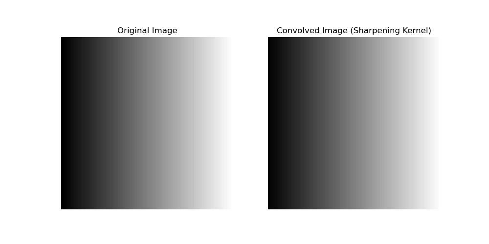
Basic Convolution with a Simple Kernel

Following is the basic example which shows how to use the scipy.ndimage.convolve() function on an image to apply convolve filter. Here in this example we apply a simple sharpening kernel to an image using scipy.ndimage.convolve() function −

import numpy as np
import matplotlib.pyplot as plt
from scipy import ndimage

# Create a simple image (e.g., a 100x100 gradient)
image = np.linspace(0, 1, 100)
image = np.tile(image, (100, 1))

# Define a simple sharpening kernel
sharpening_kernel = np.array([[0, -1, 0],
							  [-1, 5,-1],
							  [0, -1, 0]])

# Apply convolution using the kernel
convolved_image = ndimage.convolve(image, sharpening_kernel)

# Plot original and convolved images
plt.figure(figsize=(10, 5))

plt.subplot(1, 2, 1)
plt.title("Original Image")
plt.imshow(image, cmap='gray')
plt.axis('off')

plt.subplot(1, 2, 2)
plt.title("Convolved Image (Sharpening Kernel)")
plt.imshow(convolved_image, cmap='gray')
plt.axis('off')

plt.show()

Here is the output of the scipy.ndimage.convolve() function −

Convolution on larger Image

To perform convolution on a larger image, let's use a real-world image or a sample image from skimage to apply a simple kernel and visualize the result. Here in this example we will use the Sobel filter as an example to detect edges in the image by calculating the gradient of the image intensity −

import numpy as np
import matplotlib.pyplot as plt
from scipy import ndimage
from skimage import data, color

# Load a sample image (e.g., astronaut image from skimage)
image = color.rgb2gray(data.astronaut())  # Convert to grayscale

# Define the Sobel edge detection kernels (for detecting horizontal edges)
sobel_kernel_x = np.array([[-1, 0, 1],
						   [-2, 0, 2],
						   [-1, 0, 1]])

sobel_kernel_y = np.array([[-1, -2, -1],
						   [ 0,  0,  0],
						   [ 1,  2,  1]])

# Apply convolution using Sobel kernels for both x and y gradients
gradient_x = ndimage.convolve(image, sobel_kernel_x)
gradient_y = ndimage.convolve(image, sobel_kernel_y)

# Compute the magnitude of the gradients (edge strength)
edges = np.hypot(gradient_x, gradient_y)

# Plot original and edge-detected images
plt.figure(figsize=(15, 5))

plt.subplot(1, 3, 1)
plt.title("Original Image")
plt.imshow(image, cmap='gray')
plt.axis('off')

plt.subplot(1, 3, 2)
plt.title("Edges (Sobel X and Y)")
plt.imshow(edges, cmap='gray')
plt.axis('off')

plt.subplot(1, 3, 3)
plt.title("Gradient Magnitude")
plt.imshow(edges, cmap='hot')  # Hot color map to emphasize edges
plt.axis('off')

plt.show()

Here is the output of the scipy.ndimage.convolve() function applied on larger images −

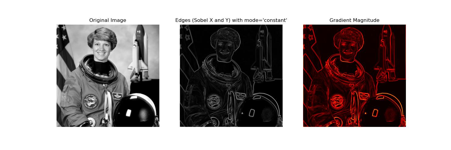
Convolution with Mode 'constant'

In convolution() function, the mode parameter controls how the boundaries of the image are handled when the kernel extends past the edges. When using mode='constant' then the areas outside the image boundaries are filled with a constant value, usually 0 is the default value −

import numpy as np
import matplotlib.pyplot as plt
from scipy import ndimage
from skimage import data, color

# Load a sample image (e.g., astronaut image from skimage)
image = color.rgb2gray(data.astronaut())  # Convert to grayscale

# Define the Sobel edge detection kernels (for detecting horizontal edges)
sobel_kernel_x = np.array([[-1, 0, 1],
						   [-2, 0, 2],
						   [-1, 0, 1]])

sobel_kernel_y = np.array([[-1, -2, -1],
						   [ 0,  0,  0],
						   [ 1,  2,  1]])

# Apply convolution using Sobel kernels for both x and y gradients with mode='constant'
gradient_x_constant = ndimage.convolve(image, sobel_kernel_x, mode='constant', cval=0.0)
gradient_y_constant = ndimage.convolve(image, sobel_kernel_y, mode='constant', cval=0.0)

# Compute the magnitude of the gradients (edge strength)
edges_constant = np.hypot(gradient_x_constant, gradient_y_constant)

# Plot original and edge-detected images
plt.figure(figsize=(15, 5))

plt.subplot(1, 3, 1)
plt.title("Original Image")
plt.imshow(image, cmap='gray')
plt.axis('off')

plt.subplot(1, 3, 2)
plt.title("Edges (Sobel X and Y) with mode='constant'")
plt.imshow(edges_constant, cmap='gray')
plt.axis('off')

plt.subplot(1, 3, 3)
plt.title("Gradient Magnitude")
plt.imshow(edges_constant, cmap='hot')  # Hot color map to emphasize edges
plt.axis('off')

plt.show()

Here is the output of the scipy.ndimage.convolve() function with constant mode −