- PyBrain - Home
- PyBrain - Overview
- PyBrain - Environment Setup
- PyBrain - Introduction to PyBrain Networks
- PyBrain - Working with Networks
- PyBrain - Working with Datasets
- PyBrain - Datasets Types
- PyBrain - Importing Data For Datasets
- PyBrain - Training Datasets on Networks
- PyBrain - Testing Network
- Working with Feed-Forward Networks
- PyBrain - Working with Recurrent Networks
- Training Network Using Optimization Algorithms
- PyBrain - Layers
- PyBrain - Connections
- PyBrain - Reinforcement Learning Module
- PyBrain - API & Tools
- PyBrain - Examples
- PyBrain Useful Resources
- PyBrain - Quick Guide
- PyBrain - Useful Resources
- PyBrain - Discussion
PyBrain - Quick Guide
PyBrain - Overview
Pybrain is an open-source library for Machine learning implemented using python. The library offers you some easy to use training algorithms for networks, datasets, trainers to train and test the network.
Definition of Pybrain as put by its official documentation is as follows −
PyBrain is a modular Machine Learning Library for Python. Its goal is to offer flexible, easy-to-use yet still powerful algorithms for Machine Learning Tasks and a variety of predefined environments to test and compare your algorithms.
PyBrain is short for Python-Based Reinforcement Learning, Artificial Intelligence, and Neural Network Library. In fact, we came up with the name first and later reverse-engineered this quite descriptive "Backronym".
Features of Pybrain
The following are the features of Pybrain −
Networks
A network is composed of modules and they are connected using connections. Pybrain supports neural networks like Feed-Forward Network, Recurrent Network, etc.
feed-forward network is a neural network, where the information between nodes moves in the forward direction and will never travel backward. Feed Forward network is the first and the simplest one among the networks available in the artificial neural network.
The information is passed from the input nodes, next to the hidden nodes and later to the output node.
Recurrent Networks are similar to Feed Forward Network; the only difference is that it has to remember the data at each step. The history of each step has to be saved.
Datasets
Datasets is the data to be given to test, validate and train on networks. The type of dataset to be used depends on the tasks that we are going to do with Machine Learning. The most commonly used datasets that Pybrain supports are SupervisedDataSet and ClassificationDataSet.
SupervisedDataSet − It consists of fields of input and target. It is the simplest form of a dataset and mainly used for supervised learning tasks.
ClassificationDataSet − It is mainly used to deal with classification problems. It takes in input, target field and also an extra field called "class" which is an automated backup of the targets given. For example, the output will be either 1 or 0 or the output will be grouped together with values based on input given, i.e., either it will fall in one particular class.
Trainer
When we create a network, i.e., neural network, it will get trained based on the training data given to it. Now whether the network is trained properly or not will depend on the prediction of test data tested on that network. The most important concept in Pybrain Training is the use of BackpropTrainer and TrainUntilConvergence.
BackpropTrainer − It is a trainer that trains the parameters of a module according to a supervised or ClassificationDataSet dataset (potentially sequential) by backpropagating the errors (through time).
TrainUntilConvergence −It is used to train the module on the dataset until it converges.
Tools
Pybrain offers tools modules which can help to build a network by importing package: pybrain.tools.shortcuts.buildNetwork
Visualization
The testing data cannot be visualized using pybrain. But Pybrain can work with other frameworks like Mathplotlib, pyplot to visualize the data.
Advantages of Pybrain
The advantages of Pybrain are −
Pybrain is an open-source free library to learn Machine Learning. It is a good start for any newcomer interested in Machine Learning.
Pybrain uses python to implement it and that makes it fast in development in comparison to languages like Java/C++.
Pybrain works easily with other libraries of python to visualize data.
Pybrain offers support for popular networks like Feed-Forward Network, Recurrent Networks, Neural Networks, etc.
Working with .csv to load datasets is very easy in Pybrain. It also allows using datasets from another library.
Training and testing of data are easy using Pybrain trainers.
Limitations of Pybrain
Pybrain offers less help for any issues faced. There are some queries unanswered on stackoverflow and on Google Group.
Workflow of Pybrain
As per Pybrain documentation the flow of machine learning is shown in the following figure −
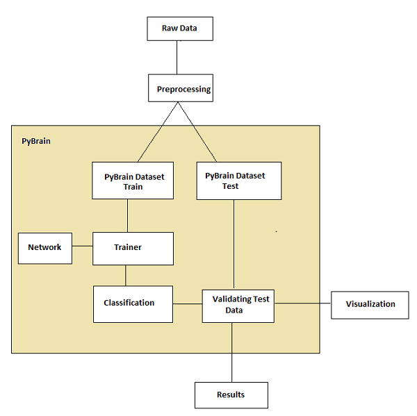
At the start, we have raw data which after preprocessing can be used with Pybrain.
The flow of Pybrain starts with datasets which are divided into trained and test data.
the network is created, and the dataset and the network are given to the trainer.
the trainer trains the data on the network and classifies the outputs as trained error and validation error which can be visualized.
the tested data can be validated to see if the output matches the trained data.
Terminology
There are important terms to be considered while working with Pybrain for machine learning. They are as follows −
Total Error − It refers to the error shown after the network is trained. If the error keeps changing on every iteration, it means it still needs time to settle, until it starts showing a constant error between iteration. Once it starts showing the constant error numbers, it means that the network has converged and will remain the same irrespective of any additional training is applied.
Trained data − It is the data used to train the Pybrain network.
Testing data − It is the data used to test the trained Pybrain network.
Trainer − When we create a network, i.e., neural network, it will get trained based on the training data given to it. Now whether the network is trained properly or not will depend on the prediction of test data tested on that network. The most important concept in Pybrain Training is the use of BackpropTrainer and TrainUntilConvergence.
BackpropTrainer − It is a trainer that trains the parameters of a module according to a supervised or ClassificationDataSet dataset (potentially sequential) by backpropagating the errors (through time).
TrainUntilConvergence − It is used to train the module on the dataset until it converges.
Layers − Layers are basically a set of functions that are used on hidden layers of a network.
Connections − A connection works similar to a layer; an only difference is that it shifts the data from one node to the other in a network.
Modules − Modules are networks which consists of input and output buffer.
Supervised Learning − In this case, we have an input and output, and we can make use of an algorithm to map the input with the output. The algorithm is made to learn on the training data given and iterated on it and the process of iteration stops when the algorithm predicts the correct data.
Unsupervised − In this case, we have input but don't know the output. The role of unsupervised learning is to get trained as much as possible with the data given.
PyBrain - Environment Setup
In this chapter, we will work on the installation of PyBrain. To start working with PyBrain, we need to install Python first. So we are going to work on following −
- Install Python
- Install PyBrain
Installing Python
To install Python, go to the Python official site: www.python.org/downloads as shown below and click on the latest version available for windows, Linux/Unix and macOS. Download Python as per your 64- or 32-bit OS available with you.

Once you have downloaded, click on the .exe file and follow the steps to install python on your system.
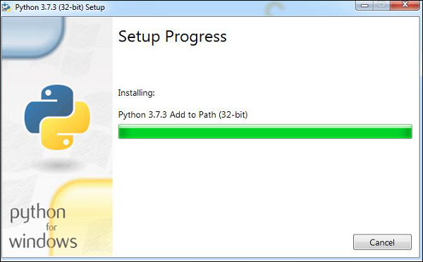
The python package manager, i.e., pip will also get installed by default with the above installation. To make it work globally on your system, directly add the location of python to the PATH variable, the same is shown at the start of the installation to remember to check the checkbox which says ADD to PATH. In case you forget to check it please follow the below given steps to add to PATH.
Add to PATH
To add to PATH, follow the below steps −
Right-click on your Computer icon and click on properties -> Advanced System Settings.
It will display the screen as shown below
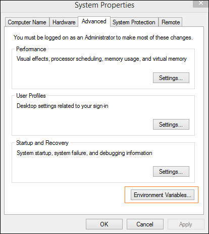
Click on Environment Variables as shown above. It will display the screen as shown below
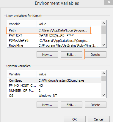
Select Path and click on Edit button, add the location path of your python at the end. Now let us check the python version.
Checking for Python version
The below code helps us in checking the version of Python −
E:\pybrain>python --version
Python 3.7.3
Installing PyBrain
Now that we have installed Python, we are going to install Pybrain. Clone the pybrain repository as shown below −
git clone git://github.com/pybrain/pybrain.git
C:\pybrain>git clone git://github.com/pybrain/pybrain.git
Cloning into 'pybrain'...
remote: Enumerating objects: 2, done.
remote: Counting objects: 100% (2/2), done.
remote: Compressing objects: 100% (2/2), done.
remote: Total 12177 (delta 0), reused 0 (delta 0), pack-reused 12175
Receiving objects: 100% (12177/12177), 13.29 MiB | 510.00 KiB/s, done.
Resolving deltas: 100% (8506/8506), done.
Now perform cd pybrain and run following command −
python setup.py install
This command will install pybrain on your system.
Once done, to check if pybrain is installed or not, open command line prompt and start the python interpreter as shown below −
C:\pybrain\pybrain>python
Python 3.7.3 (v3.7.3:ef4ec6ed12, Mar 25 2019, 22:22:05) [MSC v.1916 64 bit (AMD64)] on win32
Type "help", "copyright", "credits" or "license" for more information.
>>>
We can add import pybrain using the below code −
>>> import pybrain
>>>
If the import pybrain works without any errors, it means pybrain in installed successfully. You can now write your code to start working with pybrain.
PyBrain - Introduction to PyBrain Networks
PyBrain is a library developed for Machine Learning with Python. There are some important concepts in Machine Learning and one among them is Networks. A network is composed of modules and they are connected using connections.
A layout of a simple neural network is as follows −
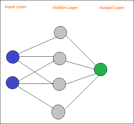
Pybrain supports neural networks such as Feed-Forward Network, Recurrent Network, etc.
A feed-forward network is a neural network, where the information between nodes moves in the forward direction and will never travel backward. Feed Forward network is the first and the simplest one among the networks available in the artificial neural network. The information is passed from the input nodes, next to the hidden nodes and later to the output node.
Here is a simple feed forward network layout.
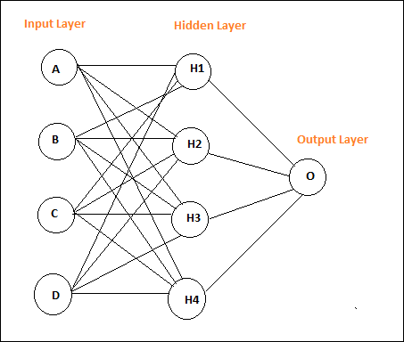
The circles are said to be modules and the lines with arrows are connections to the modules.
The nodes A, B, C and D are input nodes
H1, H2, H3, H4 are hidden nodes and O is the output.
In the above network, we have 4 input nodes, 4 hidden layers and 1 output. The number of lines shown in the diagram indicate the weight parameters in the model that are adjusted during training.
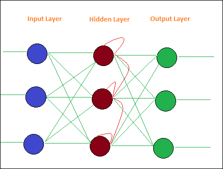
Recurrent Networks are similar to Feed Forward Network with the only difference that it has to remember the data at each step. The history of each step has to be saved.
Here is a simple Layout of Recurrent Network −
PyBrain - Working With Networks
A network is composed of modules, and they are connected using connections. In this chapter, we will learn to −
- Create Network
- Analyze Network
Creating Network
We are going to use python interpreter to execute our code. To create a network in pybrain, we have to use buildNetwork api as shown below −
C:\pybrain\pybrain>python
Python 3.7.3 (v3.7.3:ef4ec6ed12, Mar 25 2019, 22:22:05) [MSC v.1916 64 bit (AMD64)] on win32
Type "help", "copyright", "credits" or "license" for more information.
>>>
>>>
>>> from pybrain.tools.shortcuts import buildNetwork
>>> network = buildNetwork(2, 3, 1)
>>>
We have created a network using buildNetwork() and the params are 2, 3, 1 which means the network is made up of 2 inputs, 3 hidden and one single output.
Below are the details of the network, i.e., Modules and Connections −
C:\pybrain\pybrain>python
Python 3.7.3 (v3.7.3:ef4ec6ed12, Mar 25 2019, 22:22:05) [MSC v.1916 64 bit (AMD64)] on win32
Type "help", "copyright", "credits" or "license" for more information.
>>> from pybrain.tools.shortcuts import buildNetwork
>>> network = buildNetwork(2,3,1)
>>> print(network)
FeedForwardNetwork-8
   Modules:
   [<BiasUnit 'bias'>, <LinearLayer 'in'>, <SigmoidLayer 'hidden0'>,
<LinearLay er 'out'>]
   Connections:
   [<FullConnection 'FullConnection-4': 'hidden0' -> 'out'>, <FullConnection 'F
ullConnection-5': 'in' -> 'hidden0'>, <FullConnection 'FullConnection-6': 'bias'
-< 'out'>, <FullConnection 'FullConnection-7': 'bias' -> 'hidden0'>]
>>>
Modules consists of Layers, and Connection are made from FullConnection Objects. So each of the modules and connection are named as shown above.
Analyzing Network
You can access the module layers and connection individually by referring to their names as follows −
>>> network['bias']
<BiasUnit 'bias'>
>>> network['in']
<LinearLayer 'in'>
PyBrain - Working with Datasets
Datasets is an input data to be given to test, validate and train networks. The type of dataset to be used depends on the tasks that we are going to do with Machine Learning. In this chapter, we are going to take a look at the following −
- Creating Dataset
- Adding Data to Dataset
We will first learn how to create a Dataset and test the dataset with the input given.
Creating Dataset
To create a dataset we need to use the pybrain dataset package: pybrain.datasets.
Pybrain supports datasets classes like SupervisedDataset, SequentialDataset, ClassificationDataSet. We are going to make use of SupervisedDataset , to create our dataset.The dataset to be used depends on the machine learning task that user is trying to implement.SupervisedDataset is the simplest one and we are going to use the same over here.
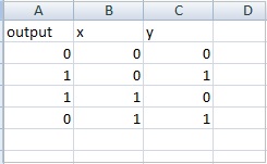
A SupervisedDataset dataset needs params input and target. Consider an XOR truth table, as shown below −
| A | B | A XOR B |
|---|---|---|
| 0 | 0 | 0 |
| 0 | 1 | 1 |
| 1 | 0 | 1 |
| 1 | 1 | 0 |
The inputs that are given are like a 2-dimensional array and we get 1 output. So here the input becomes the size and the target it the output which is 1. So the inputs that will go for our dataset will 2,1.
createdataset.py
from pybrain.datasets import SupervisedDataSet
sds = SupervisedDataSet(2, 1)
print(sds)
This is what we get when we execute above code python createdataset.py −
C:\pybrain\pybrain\src>python createdataset.py
input: dim(0, 2)
[]
target: dim(0, 1)
[]
It displays the input of size 2 and target of size 1 as shown above.
Adding Data to Dataset
Let us now add the sample data to the dataset.
createdataset.py
from pybrain.datasets import SupervisedDataSet
sds = SupervisedDataSet(2, 1)
xorModel = [
   [(0,0), (0,)],
   [(0,1), (1,)],
   [(1,0), (1,)],
   [(1,1), (0,)],
]
for input, target in xorModel:
sds.addSample(input, target)
print("Input is:")
print(sds['input'])
print("\nTarget is:")
print(sds['target'])
We have created a XORModel array as shown below −
xorModel = [
   [(0,0), (0,)],
   [(0,1), (1,)],
   [(1,0), (1,)],
   [(1,1), (0,)],
]
To add data to the dataset, we are using addSample() method which takes in input and target.
To add data to the addSample, we will loop through xorModel array as shown below −
for input, target in xorModel:
   sds.addSample(input, target)
After executing, the following is the output we get −
python createdataset.py
C:\pybrain\pybrain\src>python createdataset.py
Input is:
[[0. 0.]
[0. 1.]
[1. 0.]
[1. 1.]]
Target is:
[[0.]
[1.]
[1.]
[0.]]
You can get the input and target details from the dataset created by simply using the input and target index as shown below −
print(sds['input'])
print(sds[target])
PyBrain - Datasets Types
Datasets are data to be given to test, validate and train on networks. The type of dataset to be used depends on the tasks that we are going to do with machine learning. We are going to discuss the various dataset types in this chapter.
We can work with the dataset by adding the following package −
pybrain.dataset
SupervisedDataSet
SupervisedDataSet consists of fields of input and target. It is the simplest form of a dataset and mainly used for supervised learning tasks.
Below is how you can use it in the code −
from pybrain.datasets import SupervisedDataSet
The methods available on SupervisedDataSet are as follows −
addSample(inp, target)
This method will add a new sample of input and target.
splitWithProportion(proportion=0.10)
This will divide the datasets into two parts. The first part will have the % of the dataset given as input, i.e., if the input is .10, then it is 10% of the dataset and 90% of data. You can decide the proportion as per your choice. The divided datasets can be used for testing and training your network.
copy() − Returns a deep copy of the dataset.
clear() − Clear the dataset.
saveToFile(filename, format=None, **kwargs)
Save the object to file given by filename.
Example
Here is a working example using a SupervisedDataset −
testnetwork.py
from pybrain.tools.shortcuts import buildNetwork
from pybrain.structure import TanhLayer
from pybrain.datasets import SupervisedDataSet
from pybrain.supervised.trainers import BackpropTrainer

# Create a network with two inputs, three hidden, and one output
nn = buildNetwork(2, 3, 1, bias=True, hiddenclass=TanhLayer)

# Create a dataset that matches network input and output sizes:
norgate = SupervisedDataSet(2, 1)

# Create a dataset to be used for testing.
nortrain = SupervisedDataSet(2, 1)

# Add input and target values to dataset
# Values for NOR truth table
norgate.addSample((0, 0), (1,))
norgate.addSample((0, 1), (0,))
norgate.addSample((1, 0), (0,))
norgate.addSample((1, 1), (0,))

# Add input and target values to dataset
# Values for NOR truth table
nortrain.addSample((0, 0), (1,))
nortrain.addSample((0, 1), (0,))
nortrain.addSample((1, 0), (0,))
nortrain.addSample((1, 1), (0,))

#Training the network with dataset norgate.
trainer = BackpropTrainer(nn, norgate)

# will run the loop 1000 times to train it.
for epoch in range(1000):
   trainer.train()
trainer.testOnData(dataset=nortrain, verbose = True)
Output
The output for the above program is as follows −
python testnetwork.py
C:\pybrain\pybrain\src>python testnetwork.py
Testing on data:
('out: ', '[0.887 ]')
('correct:', '[1 ]')
error: 0.00637334
('out: ', '[0.149 ]')
('correct:', '[0 ]')
error: 0.01110338
('out: ', '[0.102 ]')
('correct:', '[0 ]')
error: 0.00522736
('out: ', '[-0.163]')
('correct:', '[0 ]')
error: 0.01328650
('All errors:', [0.006373344564625953, 0.01110338071737218, 0.005227359234093431
, 0.01328649974219942])
('Average error:', 0.008997646064572746)
('Max error:', 0.01328649974219942, 'Median error:', 0.01110338071737218)
ClassificationDataSet
This dataset is mainly used to deal with classification problems. It takes in input, target field and also an extra field called "class" which is an automated backup of the targets given. For example, the output will be either 1 or 0 or the output will be grouped together with values based on input given., i.e., it will fall in one particular class.
Here is how you can use it in the code −
from pybrain.datasets import ClassificationDataSet
Syntax
// ClassificationDataSet(inp, target=1, nb_classes=0, class_labels=None)
The methods available on ClassificationDataSet are as follows −
addSample(inp, target) − This method will add a new sample of input and target.
splitByClass() − This method will give two new datasets, the first dataset will have the class selected (0..nClasses-1), the second one will have remaining samples.
_convertToOneOfMany() − This method will convert the target classes to a 1-of-k representation, retaining the old targets as a field class
Here is a working example of ClassificationDataSet.
Example
from sklearn import datasets
import matplotlib.pyplot as plt
from pybrain.datasets import ClassificationDataSet
from pybrain.utilities import percentError
from pybrain.tools.shortcuts import buildNetwork
from pybrain.supervised.trainers import BackpropTrainer
from pybrain.structure.modules import SoftmaxLayer
from numpy import ravel
digits = datasets.load_digits()
X, y = digits.data, digits.target
ds = ClassificationDataSet(64, 1, nb_classes=10)

for i in range(len(X)):
ds.addSample(ravel(X[i]), y[i])
test_data_temp, training_data_temp = ds.splitWithProportion(0.25)
test_data = ClassificationDataSet(64, 1, nb_classes=10)

for n in range(0, test_data_temp.getLength()):
test_data.addSample( test_data_temp.getSample(n)[0], test_data_temp.getSample(n)[1] )
training_data = ClassificationDataSet(64, 1, nb_classes=10)

for n in range(0, training_data_temp.getLength()):
training_data.addSample( training_data_temp.getSample(n)[0], training_data_temp.getSample(n)[1] )
test_data._convertToOneOfMany()
training_data._convertToOneOfMany()
net = buildNetwork(training_data.indim, 64, training_data.outdim, outclass=SoftmaxLayer)
trainer = BackpropTrainer(
   net, dataset=training_data, momentum=0.1,learningrate=0.01,verbose=True,weightdecay=0.01
)
trnerr,valerr = trainer.trainUntilConvergence(dataset=training_data,maxEpochs=10)
plt.plot(trnerr,'b',valerr,'r')
plt.show()
trainer.trainEpochs(10)
print('Percent Error on testData:',percentError(trainer.testOnClassData(dataset=test_data), test_data['class']))
The dataset used in the above example is a digit dataset and the classes are from 0-9, so there are 10 classes. The input is 64, target is 1 and classes, 10.
The code trains the network with the dataset and outputs the graph for training error and validation error. It also gives the percent error on testdata which is as follows −
Output

Total error: 0.0432857814358
Total error: 0.0222276374185
Total error: 0.0149012052174
Total error: 0.011876985318
Total error: 0.00939854792853
Total error: 0.00782202445183
Total error: 0.00714707652044
Total error: 0.00606068893793
Total error: 0.00544257958975
Total error: 0.00463929281336
Total error: 0.00441275665294
('train-errors:', '[0.043286 , 0.022228 , 0.014901 , 0.011877 , 0.009399 , 0.007
   822 , 0.007147 , 0.006061 , 0.005443 , 0.004639 , 0.004413 ]')
('valid-errors:', '[0.074296 , 0.027332 , 0.016461 , 0.014298 , 0.012129 , 0.009
   248 , 0.008922 , 0.007917 , 0.006547 , 0.005883 , 0.006572 , 0.005811 ]')
Percent Error on testData: 3.34075723830735
PyBrain - Importing Data For Datasets
In this chapter, we will learn how to get data to work with Pybrain datasets.
The most commonly used are datasets are −
- Using sklearn
- From CSV file
Using sklearn
Using sklearn
Here is the link that has details of datasets from sklearn:https://scikit-learn.org/stable/datasets/toy_dataset.html
Here are a few examples of how to use datasets from sklearn −
Example 1: load_digits()
from sklearn import datasets
from pybrain.datasets import ClassificationDataSet
digits = datasets.load_digits()
X, y = digits.data, digits.target
ds = ClassificationDataSet(64, 1, nb_classes=10)
for i in range(len(X)):
ds.addSample(ravel(X[i]), y[i])
Example 2: load_iris()
from sklearn import datasets
from pybrain.datasets import ClassificationDataSet
digits = datasets.load_iris()
X, y = digits.data, digits.target
ds = ClassificationDataSet(4, 1, nb_classes=3)
for i in range(len(X)):
ds.addSample(X[i], y[i])
From CSV file
We can also use data from csv file as follows −
Here is sample data for xor truth table: datasettest.csv
Here is the working example to read the data from .csv file for dataset.
Example
from pybrain.tools.shortcuts import buildNetwork
from pybrain.structure import TanhLayer
from pybrain.datasets import SupervisedDataSet
from pybrain.supervised.trainers import BackpropTrainer
import pandas as pd

print('Read data...')
df = pd.read_csv('data/datasettest.csv',header=0).head(1000)
data = df.values

train_output = data[:,0]
train_data = data[:,1:]

print(train_output)
print(train_data)

# Create a network with two inputs, three hidden, and one output
nn = buildNetwork(2, 3, 1, bias=True, hiddenclass=TanhLayer)

# Create a dataset that matches network input and output sizes:
_gate = SupervisedDataSet(2, 1)

# Create a dataset to be used for testing.
nortrain = SupervisedDataSet(2, 1)

# Add input and target values to dataset
# Values for NOR truth table
for i in range(0, len(train_output)) :
   _gate.addSample(train_data[i], train_output[i])

#Training the network with dataset norgate.
trainer = BackpropTrainer(nn, _gate)

# will run the loop 1000 times to train it.
for epoch in range(1000):
   trainer.train()
trainer.testOnData(dataset=_gate, verbose = True)
Panda is used to read data from csv file as shown in the example.
Output
C:\pybrain\pybrain\src>python testcsv.py
Read data...
[0 1 1 0]
[
   [0 0]
   [0 1]
   [1 0]
   [1 1]
]
Testing on data:
('out: ', '[0.004 ]')
('correct:', '[0 ]')
error: 0.00000795
('out: ', '[0.997 ]')
('correct:', '[1 ]')
error: 0.00000380
('out: ', '[0.996 ]')
('correct:', '[1 ]')
error: 0.00000826
('out: ', '[0.004 ]')
('correct:', '[0 ]')
error: 0.00000829
('All errors:', [7.94733477723902e-06, 3.798267582566822e-06, 8.260969076585322e
-06, 8.286246525558165e-06])
('Average error:', 7.073204490487332e-06)
('Max error:', 8.286246525558165e-06, 'Median error:', 8.260969076585322e-06)
PyBrain - Training Datasets on Networks
So far, we have seen how to create a network and a dataset. To work with datasets and networks together, we have to do it with the help of trainers.
Below is a working example to see how to add a dataset to the network created, and later trained and tested using trainers.
testnetwork.py
from pybrain.tools.shortcuts import buildNetwork
from pybrain.structure import TanhLayer
from pybrain.datasets import SupervisedDataSet
from pybrain.supervised.trainers import BackpropTrainer

# Create a network with two inputs, three hidden, and one output
nn = buildNetwork(2, 3, 1, bias=True, hiddenclass=TanhLayer)

# Create a dataset that matches network input and output sizes:
norgate = SupervisedDataSet(2, 1)

# Create a dataset to be used for testing.
nortrain = SupervisedDataSet(2, 1)

# Add input and target values to dataset
# Values for NOR truth table
norgate.addSample((0, 0), (1,))
norgate.addSample((0, 1), (0,))
norgate.addSample((1, 0), (0,))
norgate.addSample((1, 1), (0,))

# Add input and target values to dataset
# Values for NOR truth table
nortrain.addSample((0, 0), (1,))
nortrain.addSample((0, 1), (0,))
nortrain.addSample((1, 0), (0,))
nortrain.addSample((1, 1), (0,))

#Training the network with dataset norgate.
trainer = BackpropTrainer(nn, norgate)

# will run the loop 1000 times to train it.
for epoch in range(1000):
trainer.train()
trainer.testOnData(dataset=nortrain, verbose = True)
To test the network and dataset, we need BackpropTrainer. BackpropTrainer is a trainer that trains the parameters of a module according to a supervised dataset (potentially sequential) by backpropagating the errors (through time).
We have created 2 datasets of class - SupervisedDataSet. We are making use of NOR data model which is as follows −
| A | B | A NOR B |
|---|---|---|
| 0 | 0 | 1 |
| 0 | 1 | 0 |
| 1 | 0 | 0 |
| 1 | 1 | 0 |
The above data model is used to train the network.
norgate = SupervisedDataSet(2, 1)
# Add input and target values to dataset
# Values for NOR truth table
norgate.addSample((0, 0), (1,))
norgate.addSample((0, 1), (0,))
norgate.addSample((1, 0), (0,))
norgate.addSample((1, 1), (0,))
Following is the dataset used to test −
# Create a dataset to be used for testing.
nortrain = SupervisedDataSet(2, 1)

# Add input and target values to dataset
# Values for NOR truth table
norgate.addSample((0, 0), (1,))
norgate.addSample((0, 1), (0,))
norgate.addSample((1, 0), (0,))
norgate.addSample((1, 1), (0,))
The trainer is used as follows −
#Training the network with dataset norgate.
trainer = BackpropTrainer(nn, norgate)

# will run the loop 1000 times to train it.
for epoch in range(1000):
   trainer.train()
To test on the dataset, we can use the below code −
trainer.testOnData(dataset=nortrain, verbose = True)
Output
python testnetwork.py
C:\pybrain\pybrain\src>python testnetwork.py
Testing on data:
('out: ', '[0.887 ]')
('correct:', '[1 ]')
error: 0.00637334
('out: ', '[0.149 ]')
('correct:', '[0 ]')
error: 0.01110338
('out: ', '[0.102 ]')
('correct:', '[0 ]')
error: 0.00522736
('out: ', '[-0.163]')
('correct:', '[0 ]')
error: 0.01328650
('All errors:', [0.006373344564625953, 0.01110338071737218, 0.005227359234093431
, 0.01328649974219942])
('Average error:', 0.008997646064572746)
('Max error:', 0.01328649974219942, 'Median error:', 0.01110338071737218)
If you check the output, the test data almost matches with the dataset we have provided and hence the error is 0.008.
Let us now change the test data and see an average error. We have changed the output as shown below −
Following is the dataset used to test −
# Create a dataset to be used for testing.
nortrain = SupervisedDataSet(2, 1)

# Add input and target values to dataset
# Values for NOR truth table
norgate.addSample((0, 0), (0,))
norgate.addSample((0, 1), (1,))
norgate.addSample((1, 0), (1,))
norgate.addSample((1, 1), (0,))
Let us now test it.
Output
python testnework.py
C:\pybrain\pybrain\src>python testnetwork.py
Testing on data:
('out: ', '[0.988 ]')
('correct:', '[0 ]')
error: 0.48842978
('out: ', '[0.027 ]')
('correct:', '[1 ]')
error: 0.47382097
('out: ', '[0.021 ]')
('correct:', '[1 ]')
error: 0.47876379
('out: ', '[-0.04 ]')
('correct:', '[0 ]')
error: 0.00079160
('All errors:', [0.4884297811030845, 0.47382096780393873, 0.47876378995939756, 0
.0007915982149002194])
('Average error:', 0.3604515342703303)
('Max error:', 0.4884297811030845, 'Median error:', 0.47876378995939756)
We are getting the error as 0.36, which shows that our test data is not completely matching with the network trained.
PyBrain - Testing Network
In this chapter, we are going to see some example where we are going to train the data and test the errors on the trained data.
We are going to make use of trainers −
BackpropTrainer
BackpropTrainer is trainer that trains the parameters of a module according to a supervised or ClassificationDataSet dataset (potentially sequential) by backpropagating the errors (through time).
TrainUntilConvergence
It is used to train the module on the dataset until it converges.
When we create a neural network, it will get trained based on the training data given to it.Now whether the network is trained properly or not will depend on prediction of test data tested on that network.
Let us see a working example step by step which where will build a neural network and predict the training errors, test errors and validation errors.
Testing our Network
Following are the steps we will follow for testing our Network −
- Importing required PyBrain and other packages
- Create ClassificationDataSet
- Splitting the datasets 25% as testdata and 75% as trained data
- Converting Testdata and Trained data back as ClassificationDataSet
- Creating a Neural Network
- Training the Network
- Visualizing the error and validation data
- Percentage for test data Error
Step 1
Importing required PyBrain and other packages.
The packages that we need are imported as shown below −
from sklearn import datasets
import matplotlib.pyplot as plt
from pybrain.datasets import ClassificationDataSet
from pybrain.utilities import percentError
from pybrain.tools.shortcuts import buildNetwork
from pybrain.supervised.trainers import BackpropTrainer
from pybrain.structure.modules import SoftmaxLayer
from numpy import ravel
Step 2
The next step is to create ClassificationDataSet.
For Datasets, we are going to use datasets from sklearn datasets as shown below −
Refer load_digits datasets from sklearn in the below link −
digits = datasets.load_digits()
X, y = digits.data, digits.target

ds = ClassificationDataSet(64, 1, nb_classes=10)
# we are having inputs are 64 dim array and since the digits are from 0-9 the
classes considered is 10.

for i in range(len(X)):
   ds.addSample(ravel(X[i]), y[i]) # adding sample to datasets
Step 3
Splitting the datasets 25% as testdata and 75% as trained data −
test_data_temp, training_data_temp = ds.splitWithProportion(0.25)
So here, we have used a method on dataset called splitWithProportion() with value 0.25, it will split the dataset into 25% as test data and 75% as training data.
Step 4
Converting Testdata and Trained data back as ClassificationDataSet.
test_data = ClassificationDataSet(64, 1, nb_classes=10)
for n in range(0, test_data_temp.getLength()):
   test_data.addSample( test_data_temp.getSample(n)[0], test_data_temp.getSample(n)[1] )
training_data = ClassificationDataSet(64, 1, nb_classes=10)

for n in range(0, training_data_temp.getLength()):

training_data.addSample(
   training_data_temp.getSample(n)[0], training_data_temp.getSample(n)[1]
)
test_data._convertToOneOfMany()
training_data._convertToOneOfMany()
Using splitWithProportion() method on dataset converts the dataset to superviseddataset, so we will convert the dataset back to classificationdataset as shown in above step.
Step 5
Next step is creating a Neural Network.
net = buildNetwork(training_data.indim, 64, training_data.outdim, outclass=SoftmaxLayer)
We are creating a network wherein the input and output are used from the training data.
Step 6
Training the Network
Now the important part is training the network on the dataset as shown below −
trainer = BackpropTrainer(net, dataset=training_data,
momentum=0.1,learningrate=0.01,verbose=True,weightdecay=0.01)
We are using BackpropTrainer() method and using dataset on the network created.
Step 7
The next step is visualizing the error and validation of the data.
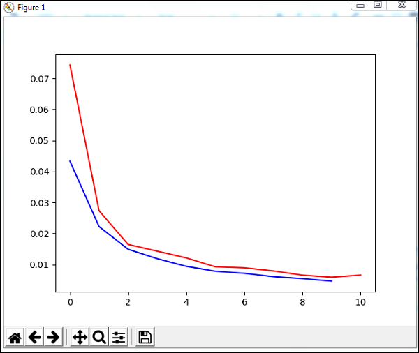
trnerr,valerr = trainer.trainUntilConvergence(dataset=training_data,maxEpochs=10)
plt.plot(trnerr,'b',valerr,'r')
plt.show()
We will use a method called trainUntilConvergence on training data that will converge for epochs of 10. It will return training error and validation error which we have plotted as shown below. The blue line shows the training errors and red line shows the validation error.
Total error received during execution of the above code is shown below −
Total error: 0.0432857814358
Total error: 0.0222276374185
Total error: 0.0149012052174
Total error: 0.011876985318
Total error: 0.00939854792853
Total error: 0.00782202445183
Total error: 0.00714707652044
Total error: 0.00606068893793
Total error: 0.00544257958975
Total error: 0.00463929281336
Total error: 0.00441275665294
('train-errors:', '[0.043286 , 0.022228 , 0.014901 , 0.011877 , 0.009399 , 0.007
822 , 0.007147 , 0.006061 , 0.005443 , 0.004639 , 0.004413 ]')
('valid-errors:', '[0.074296 , 0.027332 , 0.016461 , 0.014298 , 0.012129 , 0.009
248 , 0.008922 , 0.007917 , 0.006547 , 0.005883 , 0.006572 , 0.005811 ]')
The error starts at 0.04 and later goes down for each epoch, which means the network is getting trained and gets better for each epoch.
Step 8
Percentage for test data error
We can check the percent error using percentError method as shown below −
print('Percent Error on
   testData:',percentError(trainer.testOnClassData(dataset=test_data),
   test_data['class']))
Percent Error on testData − 3.34075723830735
We are getting the error percent, i.e., 3.34%, which means the neural network is 97% accurate.
Below is the full code −
from sklearn import datasets
import matplotlib.pyplot as plt
from pybrain.datasets import ClassificationDataSet
from pybrain.utilities import percentError
from pybrain.tools.shortcuts import buildNetwork
from pybrain.supervised.trainers import BackpropTrainer
from pybrain.structure.modules import SoftmaxLayer
from numpy import ravel
digits = datasets.load_digits()
X, y = digits.data, digits.target

ds = ClassificationDataSet(64, 1, nb_classes=10)

for i in range(len(X)):
   ds.addSample(ravel(X[i]), y[i])

test_data_temp, training_data_temp = ds.splitWithProportion(0.25)
test_data = ClassificationDataSet(64, 1, nb_classes=10)
for n in range(0, test_data_temp.getLength()):
   test_data.addSample( test_data_temp.getSample(n)[0], test_data_temp.getSample(n)[1] )
training_data = ClassificationDataSet(64, 1, nb_classes=10)

for n in range(0, training_data_temp.getLength()):
   training_data.addSample(
      training_data_temp.getSample(n)[0], training_data_temp.getSample(n)[1]
   )
test_data._convertToOneOfMany()
training_data._convertToOneOfMany()

net = buildNetwork(training_data.indim, 64, training_data.outdim, outclass=SoftmaxLayer)
trainer = BackpropTrainer(
   net, dataset=training_data, momentum=0.1,
   learningrate=0.01,verbose=True,weightdecay=0.01
)
trnerr,valerr = trainer.trainUntilConvergence(dataset=training_data,maxEpochs=10)
plt.plot(trnerr,'b',valerr,'r')
plt.show()

trainer.trainEpochs(10)
print('Percent Error on testData:',percentError(
   trainer.testOnClassData(dataset=test_data), test_data['class']
))
PyBrain - Working with Feed-Forward Networks
A feed-forward network is a neural network, where the information between nodes moves in the forward direction and will never travel backward. Feed Forward network is the first and the simplest one among the networks available in the artificial neural network. The information is passed from the input nodes, next to the hidden nodes and later to the output node.
In this chapter we are going to discuss how to −
- Create Feed-Forward Networks
- Add Connection and Modules to FFN
Creating a Feed Forward Network
You can use the python IDE of your choice, i.e., PyCharm. In this, we are using Visual Studio Code to write the code and will execute the same in terminal.
To create a feedforward network, we need to import it from pybrain.structure as shown below −
ffn.py
from pybrain.structure import FeedForwardNetwork
network = FeedForwardNetwork()
print(network)
Execute ffn.py as shown below −
C:\pybrain\pybrain\src>python ffn.py
FeedForwardNetwork-0
Modules:
[]
Connections:
[]
We have not added any modules and connections to the feedforward network. Hence the network shows empty arrays for Modules and Connections.
Adding Modules and Connections
First we will create input, hidden, output layers and add the same to the modules as shown below −
ffy.py
from pybrain.structure import FeedForwardNetwork
from pybrain.structure import LinearLayer, SigmoidLayer
network = FeedForwardNetwork()

#creating layer for input => 2 , hidden=> 3 and output=>1
inputLayer = LinearLayer(2)
hiddenLayer = SigmoidLayer(3)
outputLayer = LinearLayer(1)

#adding the layer to feedforward network
network.addInputModule(inputLayer)
network.addModule(hiddenLayer)
network.addOutputModule(outputLayer)

print(network)
Output
C:\pybrain\pybrain\src>python ffn.py
FeedForwardNetwork-3
Modules:
[]
Connections:
[]
We are still getting the modules and connections as empty. We need to provide a connection to the modules created as shown below −
Here is the code where we have created a connection between input, hidden and output layers and add the connection to the network.
ffy.py
from pybrain.structure import FeedForwardNetwork
from pybrain.structure import LinearLayer, SigmoidLayer
from pybrain.structure import FullConnection
network = FeedForwardNetwork()

#creating layer for input => 2 , hidden=> 3 and output=>1
inputLayer = LinearLayer(2)
hiddenLayer = SigmoidLayer(3)
outputLayer = LinearLayer(1)

#adding the layer to feedforward network
network.addInputModule(inputLayer)
network.addModule(hiddenLayer)
network.addOutputModule(outputLayer)

#Create connection between input ,hidden and output
input_to_hidden = FullConnection(inputLayer, hiddenLayer)
hidden_to_output = FullConnection(hiddenLayer, outputLayer)

#add connection to the network
network.addConnection(input_to_hidden)
network.addConnection(hidden_to_output)

print(network)
Output
C:\pybrain\pybrain\src>python ffn.py
FeedForwardNetwork-3
Modules:
[]
Connections:
[]
We are still not able to get the modules and connections. Let us now add the final step, i.e., we need to add the sortModules() method as shown below −
ffy.py
from pybrain.structure import FeedForwardNetwork
from pybrain.structure import LinearLayer, SigmoidLayer
from pybrain.structure import FullConnection
network = FeedForwardNetwork()

#creating layer for input => 2 , hidden=> 3 and output=>1
inputLayer = LinearLayer(2)
hiddenLayer = SigmoidLayer(3)
outputLayer = LinearLayer(1)

#adding the layer to feedforward network
network.addInputModule(inputLayer)
network.addModule(hiddenLayer)
network.addOutputModule(outputLayer)

#Create connection between input ,hidden and output
input_to_hidden = FullConnection(inputLayer, hiddenLayer)
hidden_to_output = FullConnection(hiddenLayer, outputLayer)

#add connection to the network
network.addConnection(input_to_hidden)
network.addConnection(hidden_to_output)
network.sortModules()

print(network)
Output
C:\pybrain\pybrain\src>python ffn.py
FeedForwardNetwork-6
Modules:
[<LinearLayer 'LinearLayer-3'gt;, <SigmoidLayer 'SigmoidLayer-7'>,
   <LinearLayer 'LinearLayer-8'>]
Connections:
[<FullConnection 'FullConnection-4': 'SigmoidLayer-7' -> 'LinearLayer-8'>,
   <FullConnection 'FullConnection-5': 'LinearLayer-3' -> 'SigmoidLayer-7'>]
We are now able to see the modules and the connections details for feedforwardnetwork.
PyBrain - Working with Recurrent Networks
Recurrent Networks is same as feed-forward network with only difference that you need to remember the data at each step.The history of each step has to be saved.
We will learn how to −
- Create a Recurrent Network
- Adding Modules and Connection
Creating a Recurrent Network
To create recurrent network, we will use RecurrentNetwork class as shown below −
rn.py
from pybrain.structure import RecurrentNetwork
recurrentn = RecurrentNetwork()
print(recurrentn)
python rn.py
C:\pybrain\pybrain\src>python rn.py
RecurrentNetwork-0
Modules:
[]
Connections:
[]
Recurrent Connections:
[]
We can see a new connection called Recurrent Connections for the recurrent network. Right now there is no data available.
Let us now create the layers and add to modules and create connections.
Adding Modules and Connection
We are going to create layers, i.e., input, hidden and output. The layers will be added to the input and output module. Next, we will create the connection for input to hidden, hidden to output and a recurrent connection between hidden to hidden.
Here is the code for the Recurrent network with modules and connections.
rn.py
from pybrain.structure import RecurrentNetwork
from pybrain.structure import LinearLayer, SigmoidLayer
from pybrain.structure import FullConnection
recurrentn = RecurrentNetwork()

#creating layer for input => 2 , hidden=> 3 and output=>1
inputLayer = LinearLayer(2, 'rn_in')
hiddenLayer = SigmoidLayer(3, 'rn_hidden')
outputLayer = LinearLayer(1, 'rn_output')

#adding the layer to feedforward network
recurrentn.addInputModule(inputLayer)
recurrentn.addModule(hiddenLayer)
recurrentn.addOutputModule(outputLayer)

#Create connection between input ,hidden and output
input_to_hidden = FullConnection(inputLayer, hiddenLayer)
hidden_to_output = FullConnection(hiddenLayer, outputLayer)
hidden_to_hidden = FullConnection(hiddenLayer, hiddenLayer)

#add connection to the network
recurrentn.addConnection(input_to_hidden)
recurrentn.addConnection(hidden_to_output)
recurrentn.addRecurrentConnection(hidden_to_hidden)
recurrentn.sortModules()

print(recurrentn)
python rn.py
C:\pybrain\pybrain\src>python rn.py
RecurrentNetwork-6
Modules:
[<LinearLayer 'rn_in'>, <SigmoidLayer 'rn_hidden'>,
   <LinearLayer 'rn_output'>]
Connections:
[<FullConnection 'FullConnection-4': 'rn_hidden' -> 'rn_output'>,
   <FullConnection 'FullConnection-5': 'rn_in' -> 'rn_hidden'>]
Recurrent Connections:
[<FullConnection 'FullConnection-3': 'rn_hidden' -> 'rn_hidden'>]
In above ouput we can see the Modules, Connections and Recurrent Connections.
Let us now activate the network using activate method as shown below −
rn.py
Add below code to the one created earlier −
#activate network using activate() method
act1 = recurrentn.activate((2, 2))
print(act1)

act2 = recurrentn.activate((2, 2))
print(act2)
python rn.py
C:\pybrain\pybrain\src>python rn.py
[-1.24317586]
[-0.54117783]
Training Network Using Optimization Algorithms
We have seen how to train a network using trainers in pybrain. In this chapter, will use optimization algorithms available with Pybrain to train a network.
In the example, we will use the GA optimization algorithm which needs to be imported as shown below −
from pybrain.optimization.populationbased.ga import GA
Example
Below is a working example of a training network using a GA optimization algorithm −
from pybrain.datasets.classification import ClassificationDataSet
from pybrain.optimization.populationbased.ga import GA
from pybrain.tools.shortcuts import buildNetwork

# create XOR dataset
ds = ClassificationDataSet(2)
ds.addSample([0., 0.], [0.])
ds.addSample([0., 1.], [1.])
ds.addSample([1., 0.], [1.])
ds.addSample([1., 1.], [0.])
ds.setField('class', [ [0.],[1.],[1.],[0.]])

net = buildNetwork(2, 3, 1)
ga = GA(ds.evaluateModuleMSE, net, minimize=True)

for i in range(100):
net = ga.learn(0)[0]

print(net.activate([0,0]))
print(net.activate([1,0]))
print(net.activate([0,1]))
print(net.activate([1,1]))
Output
The activate method on the network for the inputs almost matches with the output as shown below −
C:\pybrain\pybrain\src>python example15.py
[0.03055398]
[0.92094839]
[1.12246157]
[0.02071285]
PyBrain - Layers
Layers are basically a set of functions that are used on hidden layers of a network.
We will go through the following details about layers in this chapter −
- Understanding layer
- Creating Layer using Pybrain
Understanding layers
We have seen examples earlier where we have used layers as follows −
- TanhLayer
- SoftmaxLayer
Example using TanhLayer
Below is one example where we have used TanhLayer for building a network −
testnetwork.py
from pybrain.tools.shortcuts import buildNetwork
from pybrain.structure import TanhLayer
from pybrain.datasets import SupervisedDataSet
from pybrain.supervised.trainers import BackpropTrainer

# Create a network with two inputs, three hidden, and one output
nn = buildNetwork(2, 3, 1, bias=True, hiddenclass=TanhLayer)

# Create a dataset that matches network input and output sizes:
norgate = SupervisedDataSet(2, 1)

# Create a dataset to be used for testing.
nortrain = SupervisedDataSet(2, 1)

# Add input and target values to dataset
# Values for NOR truth table
norgate.addSample((0, 0), (1,))
norgate.addSample((0, 1), (0,))
norgate.addSample((1, 0), (0,))
norgate.addSample((1, 1), (0,))

# Add input and target values to dataset
# Values for NOR truth table
nortrain.addSample((0, 0), (1,))
nortrain.addSample((0, 1), (0,))
nortrain.addSample((1, 0), (0,))
nortrain.addSample((1, 1), (0,))

#Training the network with dataset norgate.
trainer = BackpropTrainer(nn, norgate)

# will run the loop 1000 times to train it.
for epoch in range(1000):
   trainer.train()
trainer.testOnData(dataset=nortrain, verbose = True)
Output
The output for the above code is as follows −
python testnetwork.py
C:\pybrain\pybrain\src>python testnetwork.py
Testing on data:
('out: ', '[0.887 ]')
('correct:', '[1 ]')
error: 0.00637334
('out: ', '[0.149 ]')
('correct:', '[0 ]')
error: 0.01110338
('out: ', '[0.102 ]')
('correct:', '[0 ]')
error: 0.00522736
('out: ', '[-0.163]')
('correct:', '[0 ]')
error: 0.01328650
('All errors:', [0.006373344564625953, 0.01110338071737218,
   0.005227359234093431, 0.01328649974219942])
('Average error:', 0.008997646064572746)
('Max error:', 0.01328649974219942, 'Median error:', 0.01110338071737218)
Example using SoftMaxLayer
Below is one example where we have used SoftmaxLayer for building a network −
from pybrain.tools.shortcuts import buildNetwork
from pybrain.structure.modules import SoftmaxLayer
from pybrain.datasets import SupervisedDataSet
from pybrain.supervised.trainers import BackpropTrainer

# Create a network with two inputs, three hidden, and one output
nn = buildNetwork(2, 3, 1, bias=True, hiddenclass=SoftmaxLayer)

# Create a dataset that matches network input and output sizes:
norgate = SupervisedDataSet(2, 1)

# Create a dataset to be used for testing.
nortrain = SupervisedDataSet(2, 1)

# Add input and target values to dataset
# Values for NOR truth table
norgate.addSample((0, 0), (1,))
norgate.addSample((0, 1), (0,))
norgate.addSample((1, 0), (0,))
norgate.addSample((1, 1), (0,))

# Add input and target values to dataset
# Values for NOR truth table
nortrain.addSample((0, 0), (1,))
nortrain.addSample((0, 1), (0,))
nortrain.addSample((1, 0), (0,))
nortrain.addSample((1, 1), (0,))

#Training the network with dataset norgate.
trainer = BackpropTrainer(nn, norgate)

# will run the loop 1000 times to train it.
for epoch in range(1000):
trainer.train()
trainer.testOnData(dataset=nortrain, verbose = True)
Output
The output is as follows −
C:\pybrain\pybrain\src>python example16.py
Testing on data:
('out: ', '[0.918 ]')
('correct:', '[1 ]')
error: 0.00333524
('out: ', '[0.082 ]')
('correct:', '[0 ]')
error: 0.00333484
('out: ', '[0.078 ]')
('correct:', '[0 ]')
error: 0.00303433
('out: ', '[-0.082]')
('correct:', '[0 ]')
error: 0.00340005
('All errors:', [0.0033352368788838365, 0.003334842961037291,
   0.003034328685718761, 0.0034000458892589056])
('Average error:', 0.0032761136037246985)
('Max error:', 0.0034000458892589056, 'Median error:', 0.0033352368788838365)
Creating Layer in Pybrain
In Pybrain, you can create your own layer as follows −
To create a layer, you need to use NeuronLayer class as the base class to create all type of layers.
Example
from pybrain.structure.modules.neuronlayer import NeuronLayer
class LinearLayer(NeuronLayer):
   def _forwardImplementation(self, inbuf, outbuf):
      outbuf[:] = inbuf
   def _backwardImplementation(self, outerr, inerr, outbuf, inbuf):
      inerr[:] = outer
To create a Layer, we need to implement two methods: _forwardImplementation() and _backwardImplementation().
The _forwardImplementation() takes in 2 arguments inbuf and outbuf, which are Scipy arrays. Its size is dependent on the layers input and output dimensions.
The _backwardImplementation() is used to calculate the derivative of the output with respect to the input given.
So to implement a layer in Pybrain, this is the skeleton of the layer class −
from pybrain.structure.modules.neuronlayer import NeuronLayer
class NewLayer(NeuronLayer):
   def _forwardImplementation(self, inbuf, outbuf):
      pass
   def _backwardImplementation(self, outerr, inerr, outbuf, inbuf):
      pass
In case you want to implement a quadratic polynomial function as a layer, we can do so as follows −
Consider we have a polynomial function as −
f(x) = 3x2
The derivative of the above polynomial function will be as follows −
f(x) = 6 x
The final layer class for the above polynomial function will be as follows −
testlayer.py
from pybrain.structure.modules.neuronlayer import NeuronLayer
class PolynomialLayer(NeuronLayer):
   def _forwardImplementation(self, inbuf, outbuf):
      outbuf[:] = 3*inbuf**2
   def _backwardImplementation(self, outerr, inerr, outbuf, inbuf):
      inerr[:] = 6*inbuf*outerr
Now let us make use of the layer created as shown below −
testlayer1.py
from testlayer import PolynomialLayer
from pybrain.tools.shortcuts import buildNetwork
from pybrain.tests.helpers import gradientCheck

n = buildNetwork(2, 3, 1, hiddenclass=PolynomialLayer)
n.randomize()

gradientCheck(n)
GradientCheck() will test whether the layer is working fine or not.We need to pass the network where the layer is used to gradientCheck(n).It will give the output as Perfect Gradient if the layer is working fine.
Output
C:\pybrain\pybrain\src>python testlayer1.py
Perfect gradient
PyBrain - Connections
A connection works similar to a layer; an only difference is that it shifts the data from one node to the other in a network.
In this chapter, we are going to learn about −
- Understanding Connections
- Creating Connections
Understanding Connections
Here is a working example of connections used while creating a network.
Example
ffy.py
from pybrain.structure import FeedForwardNetwork
from pybrain.structure import LinearLayer, SigmoidLayer
from pybrain.structure import FullConnection

network = FeedForwardNetwork()

#creating layer for input => 2 , hidden=> 3 and output=>1
inputLayer = LinearLayer(2)
hiddenLayer = SigmoidLayer(3)
outputLayer = LinearLayer(1)

#adding the layer to feedforward network
network.addInputModule(inputLayer)
network.addModule(hiddenLayer)
network.addOutputModule(outputLayer)

#Create connection between input ,hidden and output
input_to_hidden = FullConnection(inputLayer, hiddenLayer)
hidden_to_output = FullConnection(hiddenLayer, outputLayer)

#add connection to the network
network.addConnection(input_to_hidden)
network.addConnection(hidden_to_output)
network.sortModules()

print(network)
Output
C:\pybrain\pybrain\src>python ffn.py
FeedForwardNetwork-6
Modules:
[<LinearLayer 'LinearLayer-3'>, <SigmoidLayer 'SigmoidLayer-7'>,
   <LinearLayer 'LinearLayer-8'>]
Connections:
[<FullConnection 'FullConnection-4': 'SigmoidLayer-7' -> 'LinearLayer-8'>,
   <FullConnection 'FullConnection-5': 'LinearLayer-3' -> 'SigmoidLayer-7'>]
Creating Connections
In Pybrain, we can create connections by using the connection module as shown below −
Example
connect.py
from pybrain.structure.connections.connection import Connection
class YourConnection(Connection):
   def __init__(self, *args, **kwargs):
      Connection.__init__(self, *args, **kwargs)
   def _forwardImplementation(self, inbuf, outbuf):
      outbuf += inbuf
   def _backwardImplementation(self, outerr, inerr, inbuf):
      inerr += outer
To create a connection, there are 2 methods _forwardImplementation() and _backwardImplementation().
The _forwardImplementation() is called with the output buffer of the incoming module which is inbuf, and the input buffer of the outgoing module called outbuf. The inbuf is added to the outgoing module outbuf.
The _backwardImplementation() is called with outerr, inerr, and inbuf. The outgoing module error is added to the incoming module error in _backwardImplementation().
Let us now use the YourConnection in a network.
testconnection.py
from pybrain.structure import FeedForwardNetwork
from pybrain.structure import LinearLayer, SigmoidLayer
from connect import YourConnection

network = FeedForwardNetwork()

#creating layer for input => 2 , hidden=> 3 and output=>1
inputLayer = LinearLayer(2)
hiddenLayer = SigmoidLayer(3)
outputLayer = LinearLayer(1)

#adding the layer to feedforward network
network.addInputModule(inputLayer)
network.addModule(hiddenLayer)
network.addOutputModule(outputLayer)

#Create connection between input ,hidden and output
input_to_hidden = YourConnection(inputLayer, hiddenLayer)
hidden_to_output = YourConnection(hiddenLayer, outputLayer)

#add connection to the network
network.addConnection(input_to_hidden)
network.addConnection(hidden_to_output)
network.sortModules()

print(network)
Output
C:\pybrain\pybrain\src>python testconnection.py
FeedForwardNetwork-6
Modules:
[<LinearLayer 'LinearLayer-3'>, <SigmoidLayer 'SigmoidLayer-7'>,
   <LinearLayer 'LinearLayer-8'>]
Connections:
[<YourConnection 'YourConnection-4': 'LinearLayer-3' -> 'SigmoidLayer-7'>,
   <YourConnection 'YourConnection-5': 'SigmoidLayer-7' -> 'LinearLayer-8'>]
PyBrain - Reinforcement Learning Module
Reinforcement Learning (RL) is an important part in Machine Learning. Reinforcement learning makes the agent learn its behaviour based on inputs from the environment.
The components that interact with each other during Reinforcement are as follows −
- Environment
- Agent
- Task
- Experiment
The layout of Reinforcement Learning is given below −
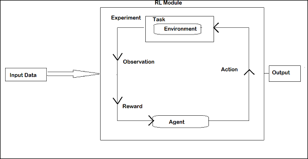
In RL, the agent talks with the environment in iteration. At each iteration, the agent receives an observation which has the reward. It then chooses the action and sends to the environment. The environment at each iteration moves to a new state and the reward received each time is saved.
The goal of RL agent is to collect as many rewards as possible. In between the iteration the agent's performance is compared with that of the agent that acts in a good way and the difference in performance gives rise to either reward or failure. RL is basically used in problem solving tasks like robot control, elevator, telecommunications, games etc.
Let us take a look at how to work with RL in Pybrain.
We are going to work on maze environment which will be represented using 2 dimensional numpy array where 1 is a wall and 0 is a free field. The agent's responsibility is to move over the free field and find the goal point.
Here is a step by step flow of working with maze environment.
Step 1
Import the packages we need with the below code −
from scipy import *
import sys, time
import matplotlib.pyplot as pylab # for visualization we are using mathplotlib

from pybrain.rl.environments.mazes import Maze, MDPMazeTask
from pybrain.rl.learners.valuebased import ActionValueTable
from pybrain.rl.agents import LearningAgent
from pybrain.rl.learners import Q, QLambda, SARSA #@UnusedImport
from pybrain.rl.explorers import BoltzmannExplorer #@UnusedImport
from pybrain.rl.experiments import Experiment
from pybrain.rl.environments import Task
Step 2
Create the maze environment using the below code −
# create the maze with walls as 1 and 0 is a free field
mazearray = array(
   [[1, 1, 1, 1, 1, 1, 1, 1, 1],
   [1, 0, 0, 1, 0, 0, 0, 0, 1],
   [1, 0, 0, 1, 0, 0, 1, 0, 1],
   [1, 0, 0, 1, 0, 0, 1, 0, 1],
   [1, 0, 0, 1, 0, 1, 1, 0, 1],
   [1, 0, 0, 0, 0, 0, 1, 0, 1],
   [1, 1, 1, 1, 1, 1, 1, 0, 1],
   [1, 0, 0, 0, 0, 0, 0, 0, 1],
   [1, 1, 1, 1, 1, 1, 1, 1, 1]]
)
env = Maze(mazearray, (7, 7)) # create the environment, the first parameter is the
maze array and second one is the goal field tuple
Step 3
The next step is to create Agent.
Agent plays an important role in RL. It will interact with the maze environment using getAction() and integrateObservation() methods.
The agent has a controller (which will map the states to actions) and a learner.
The controller in PyBrain is like a module, for which the input is states and convert them into actions.
controller = ActionValueTable(81, 4)
controller.initialize(1.)
The ActionValueTable needs 2 inputs, i.e., the number of states and actions. The standard maze environment has 4 actions: north, south, east, west.
Now we will create a learner. We are going to use SARSA() learning algorithm for the learner to be used with the agent.
learner = SARSA()
agent = LearningAgent(controller, learner)
Step 4
This step is adding Agent to Environment.
To connect the agent to environment, we need a special component called task. The role of a task is to look for the goal in the environment and how the agent gets rewards for actions.
The environment has its own task. The Maze environment that we have used has MDPMazeTask task. MDP stands for markov decision process which means, the agent knows its position in the maze. The environment will be a parameter to the task.
task = MDPMazeTask(env)
Step 5
The next step after adding agent to environment is to create an Experiment.
Now we need to create the experiment, so that we can have the task and the agent co-ordinate with each other.
experiment = Experiment(task, agent)
Now we are going to run the experiment 1000 times as shown below −
for i in range(1000):
   experiment.doInteractions(100)
   agent.learn()
   agent.reset()
The environment will run for 100 times between the agent and task when the following code gets executed −
experiment.doInteractions(100)
After each iteration, it gives back a new state to the task which decides what information and reward should be passed to the agent. We are going to plot a new table after learning and resetting the agent inside the for loop.
for i in range(1000):
   experiment.doInteractions(100)
   agent.learn()
   agent.reset()
   pylab.pcolor(table.params.reshape(81,4).max(1).reshape(9,9))
   pylab.savefig("test.png")
Here is the full code −
Example
maze.py
from scipy import *
import sys, time
import matplotlib.pyplot as pylab

from pybrain.rl.environments.mazes import Maze, MDPMazeTask
from pybrain.rl.learners.valuebased import ActionValueTable
from pybrain.rl.agents import LearningAgent
from pybrain.rl.learners import Q, QLambda, SARSA #@UnusedImport
from pybrain.rl.explorers import BoltzmannExplorer #@UnusedImport
from pybrain.rl.experiments import Experiment
from pybrain.rl.environments import Task

# create maze array
mazearray = array(
   [[1, 1, 1, 1, 1, 1, 1, 1, 1],
   [1, 0, 0, 1, 0, 0, 0, 0, 1],
   [1, 0, 0, 1, 0, 0, 1, 0, 1],
   [1, 0, 0, 1, 0, 0, 1, 0, 1],
   [1, 0, 0, 1, 0, 1, 1, 0, 1],
   [1, 0, 0, 0, 0, 0, 1, 0, 1],
   [1, 1, 1, 1, 1, 1, 1, 0, 1],
   [1, 0, 0, 0, 0, 0, 0, 0, 1],
   [1, 1, 1, 1, 1, 1, 1, 1, 1]]
)
env = Maze(mazearray, (7, 7))

# create task
task = MDPMazeTask(env)

#controller in PyBrain is like a module, for which the input is states and
convert them into actions.
controller = ActionValueTable(81, 4)
controller.initialize(1.)

# create agent with controller and learner - using SARSA()
learner = SARSA()

# create agent
agent = LearningAgent(controller, learner)

# create experiment
experiment = Experiment(task, agent)

# prepare plotting
pylab.gray()
pylab.ion()

for i in range(1000):
experiment.doInteractions(100)

agent.learn()
agent.reset()

pylab.pcolor(controller.params.reshape(81,4).max(1).reshape(9,9))
pylab.savefig("test.png")
Output
python maze.py
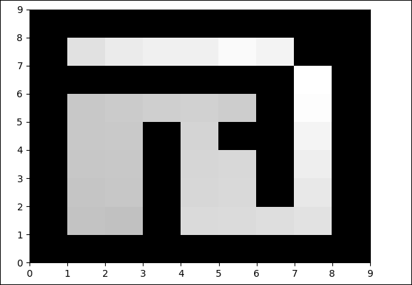
The color in the free field will be changed at each iteration.
PyBrain - API & Tools
Now we know how to build a network and train it. In this chapter, we will understand how to create and save the network, and use the network whenever required.
Save and Recover Network
We are going to make use of NetworkWriter and NetworkReader from Pybrain tool, i.e., pybrain.tools.customxml.
Here is a working example of the same −
from pybrain.tools.shortcuts import buildNetwork
from pybrain.tools.customxml import NetworkWriter
from pybrain.tools.customxml import NetworkReader

net = buildNetwork(2,1,1)
NetworkWriter.writeToFile(net, 'network.xml')
net = NetworkReader.readFrom('network.xml')
The network is saved inside network.xml.
NetworkWriter.writeToFile(net, 'network.xml')
To read the xml when required we can use code as follows −
net = NetworkReader.readFrom('network.xml')
Here is the network.xml file created −
<?xml version="1.0" ?>
<PyBrain>
   <Network class="pybrain.structure.networks.feedforward.FeedForwardNetwork" name="FeedForwardNetwork-8">
      <name val="'FeedForwardNetwork-8'"/>
      <Modules>
         <LinearLayer class="pybrain.structure.modules.linearlayer.LinearLayer" inmodule="True" name="in">
            <name val="'in'"/>
            <dim val="2"/>
         </LinearLayer>

         <LinearLayer class="pybrain.structure.modules.linearlayer.LinearLayer" name="out" outmodule="True">
            <name val="'out'"/>
            <dim val="1"/>
         </LinearLayer>

         <BiasUnit class="pybrain.structure.modules.biasunit.BiasUnit" name="bias">
            <name val="'bias'"/>
         </BiasUnit>

         <SigmoidLayer class="pybrain.structure.modules.sigmoidlayer.SigmoidLayer" name="hidden0">
            <name val="'hidden0'"/>
            <dim val="1"/>
         </SigmoidLayer>
      </Modules>

      <Connections>
         <FullConnection class="pybrain.structure.connections.full.FullConnection" name="FullConnection-6">
            <inmod val="bias"/>
            <outmod val="out"/>
            <Parameters>[1.2441093186965146]</Parameters>
         </FullConnection>

         <FullConnection class="pybrain.structure.connections.full.FullConnection" name="FullConnection-7">
            <inmod val="bias"/>
            <outmod val="hidden0"/>
            <Parameters>[-1.5743530012126412]</Parameters>
         </FullConnection>

         <FullConnection class="pybrain.structure.connections.full.FullConnection" name="FullConnection-4">
            <inmod val="in"/>
            <outmod val="hidden0"/>
            <Parameters>[-0.9429546042034236, -0.09858196752687162]</Parameters>
         </FullConnection>

         <FullConnection class="pybrain.structure.connections.full.FullConnection" name="FullConnection-5">
            <inmod val="hidden0"/>
            <outmod val="out"/>
            <Parameters>[-0.29205472354634304]</Parameters>
         </FullConnection>
      </Connections>

   </Network>
</PyBrain>
API
Below is a list of APIs that we have used throughout this tutorial.
For Networks
activate(input) − It takes parameter, i.e., the value to be tested. It will return back the result based on the input given.
activateOnDataset(dataset) − It will iterate over the dataset given and return the output.
addConnection(c) − Adds connection to the network.
addInputModule(m) − Adds the module given to the network and mark it as an input module.
addModule(m) − Adds the given module to the network.
addOutputModule(m) − Adds the module to the network and mark it as an output module.
reset() − Resets the modules and the network.
sortModules() − It prepares the network for activation by sorting internally. It has to be called before activation.
For Supervised Datasets
addSample(inp, target) − Adds a new sample of input and target.
splitWithProportion(proportion=0.5) − Divides dataset into two parts, the first part containing the proportion part data and the next set containing the remaining one.
For Trainers
trainUntilConvergence(dataset=None, maxEpochs=None, verbose=None, continueEpochs=10, validationProportion=0.25) − It is used to train the module on the dataset until it converges. If dataset is not given, it will try to train on the trained dataset used at the start.
PyBrain - Examples
In this chapter, all possible examples which are executed using PyBrain are listed.
Example 1
Working with NOR Truth Table and testing it for correctness.
from pybrain.tools.shortcuts import buildNetwork
from pybrain.structure import TanhLayer
from pybrain.datasets import SupervisedDataSet
from pybrain.supervised.trainers import BackpropTrainer

# Create a network with two inputs, three hidden, and one output
nn = buildNetwork(2, 3, 1, bias=True, hiddenclass=TanhLayer)

# Create a dataset that matches network input and output sizes:
norgate = SupervisedDataSet(2, 1)

# Create a dataset to be used for testing.
nortrain = SupervisedDataSet(2, 1)

# Add input and target values to dataset
# Values for NOR truth table
norgate.addSample((0, 0), (1,))
norgate.addSample((0, 1), (0,))
norgate.addSample((1, 0), (0,))
norgate.addSample((1, 1), (0,))

# Add input and target values to dataset
# Values for NOR truth table
nortrain.addSample((0, 0), (1,))
nortrain.addSample((0, 1), (0,))
nortrain.addSample((1, 0), (0,))
nortrain.addSample((1, 1), (0,))

#Training the network with dataset norgate.
trainer = BackpropTrainer(nn, norgate)

# will run the loop 1000 times to train it.
for epoch in range(1000):
   trainer.train()
trainer.testOnData(dataset=nortrain, verbose = True)
Output
C:\pybrain\pybrain\src>python testnetwork.py
Testing on data:
('out: ', '[0.887 ]')
('correct:', '[1 ]')
error: 0.00637334
('out: ', '[0.149 ]')
('correct:', '[0 ]')
error: 0.01110338
('out: ', '[0.102 ]')
('correct:', '[0 ]')
error: 0.00522736
('out: ', '[-0.163]')
('correct:', '[0 ]')
error: 0.01328650
('All errors:', [0.006373344564625953, 0.01110338071737218,
   0.005227359234093431, 0.01328649974219942])
('Average error:', 0.008997646064572746)
('Max error:', 0.01328649974219942, 'Median error:', 0.01110338071737218)
Example 2
For Datasets, we are going to use datasets from sklearn datasets as shown below: Refer load_digits datasets from sklearn: scikit-learn.org
It has 10 classes, i.e., digits to be predicted from 0-9.
The total input data in X is 64.
from sklearn import datasets
import matplotlib.pyplot as plt

from pybrain.datasets import ClassificationDataSet
from pybrain.utilities import percentError
from pybrain.tools.shortcuts import buildNetwork
from pybrain.supervised.trainers import BackpropTrainer
from pybrain.structure.modules import SoftmaxLayer
from numpy import ravel

digits = datasets.load_digits()
X, y = digits.data, digits.target
ds = ClassificationDataSet(64, 1, nb_classes=10) )

# we are having inputs are 64 dim array and since the digits are from 0-9
the classes considered is 10.

for i in range(len(X)):
ds.addSample(ravel(X[i]), y[i]) # adding sample to datasets
test_data_temp, training_data_temp = ds.splitWithProportion(0.25)

#Splitting the datasets 25% as testdata and 75% as trained data
# Using splitWithProportion() method on dataset converts the dataset to
#superviseddataset, so we will convert the dataset back to classificationdataset
#as shown in above step.
test_data = ClassificationDataSet(64, 1, nb_classes=10)

for n in range(0, test_data_temp.getLength()):
test_data.addSample( test_data_temp.getSample(n)[0], test_data_temp.getSample(n)[1] )
training_data = ClassificationDataSet(64, 1, nb_classes=10)

for n in range(0, training_data_temp.getLength()):
training_data.addSample(
   training_data_temp.getSample(n)[0], training_data_temp.getSample(n)[1]
)
test_data._convertToOneOfMany()
training_data._convertToOneOfMany()
net = buildNetwork(
   training_data.indim, 64, training_data.outdim, outclass=SoftmaxLayer
)
#creating a network wherein the input and output are used from the training data.
trainer = BackpropTrainer(
   net, dataset=training_data, momentum=0.1,learningrate=0.01,verbose=True,weightdecay=0.01
)
#Training the Network
trnerr,valerr = trainer.trainUntilConvergence(dataset=training_data,maxEpochs=10)

#Visualizing the error and validation data
plt.plot(trnerr,'b',valerr,'r')
plt.show()
trainer.trainEpochs(10)
print('Percent Error on testData:',percentError(
   trainer.testOnClassData(dataset=test_data), test_data['class']
))
Output

Total error: 0.0432857814358
Total error: 0.0222276374185
Total error: 0.0149012052174
Total error: 0.011876985318
Total error: 0.00939854792853
Total error: 0.00782202445183
Total error: 0.00714707652044
Total error: 0.00606068893793
Total error: 0.00544257958975
Total error: 0.00463929281336
Total error: 0.00441275665294
('train-errors:', '[0.043286 , 0.022228 , 0.014901 , 0.011877 , 0.009399 , 0.007
   822 , 0.007147 , 0.006061 , 0.005443 , 0.004639 , 0.004413 ]')
('valid-errors:', '[0.074296 , 0.027332 , 0.016461 , 0.014298 , 0.012129 , 0.009
   248 , 0.008922 , 0.007917 , 0.006547 , 0.005883 , 0.006572 , 0.005811 ]')
Percent Error on testData: 3.34075723830735
