- Multimedia - Home
- Multimedia - Introduction
- Multimedia - Systems
- Multimedia - Authoring
- Multimedia - Images & Graphics
- Multimedia - Sound & Audio
- Multimedia - Digital Audio Coding
- Multimedia Useful Resources
- Multimedia - Quick Guide
- Multimedia - Useful Resources
Multimedia Digital Audio Coding
Audio coding is used to obtain compact digital representations of high fidelity audio signals for the purpose of efficient transmission of signal or storage of signal. Objective in audio coding is to represent the signal with minimum number of bits while achieving transparent signal reproduction that is generating output audio that cannot be distinguished from the original input.
Pulse Code Modulation (PCM)
PCM is a method or technique for transmitting analog data in a digital and binary way independent of the complexity of the analog waveform.All types of analog data like video, voice; music etc. can be transferred using PCM. It is the standard form for digital audio in computers. It is used by Blu-ray, DVD and Compact Disc formats and other systemds such as digital telephone systems. PCM consists of three steps to digitize an analog signal.
Sampling
Sampling is the process of reading the values of the filtered analog signal at regular intervals. Suppose analog signal is sampled every Ts seconds. Ts are referred to as the sampling interval.
It is called the sampling rate or sampling frequency.
Quantization
Quantization is the process of assigning a discrete value from a range of possible values to each obtained sample. Possible values will depend on the number of bits used to represent each sample. Quantization can be achieved by either rounding the signal up and down to the nearest available value which is lower than the actual sample. The difference between the sample and the value assigned to it is known as the quantization noise or quantization error. Quantization noise can be reduced by increasing the number of quantization intervals or levels because the difference between the input signal amplitude and the quantization interval decreases as the number of quantization intervals increases.
Binary Encoding
Binary encoding is the process of representing the sampled values as a binary number in the range 0 to n. The value of n is choosen as a power of 2, considering the accuracy.
Differential Coding
Differential coding operates by making numbers small. Smaller numbers require less information to code than larger numbers. It would be more accurate to claim that similar numbers require less information to code. Suppose you are working with a string of bytes. Bytes range from 0.255. Here is a string:
On the scale of 0...255, those numbers are reasonably large. They are quite similar to each other. Differences are taken and coded instead of complete numbers. Normally first number is taken as such and then differences are computed.
Thus coding string of numbers is
When decoding this string of numbers, start with the first number and start adding the deltas to get the remaining numbers:
Therefore, audio is not stored in simple PCM but in a form that exploits differences.
Lossless Predictive Coding
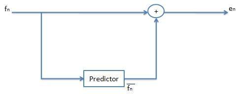
Predictive coding is based on the principle that most source or analog signals show significant correlation between successive samples so encoding uses redundancy in sample values which implies lower bit rate. Therefore, in case of predictive coding, we have to predict current sample value based upon previous samples and we have to encode the difference between actual value of sample and predicted value. The difference between actual and predicted samples is known as prediction error. Therefore, predicting coding consists of finding differences and transmitting these using a PCM system.
Assume that input signal (or samples) as the set of integer values fn. Then we predict integer value f¯n as simply the previous value. Therefore
We would like our error value en to be as small as possible. Therefore we would wish our pprediction fn to be as close as possible to the actual signal fn.
But for a particular sequence of signal values, more than one previous values fn-1,fn-2,fn-3 and so on may provide a better prediction of fn
f¯n is the mean of previous two values. Such a predictor can be followed by a truncating or rounding operation to result in integer.
Differential Pulse Code Modulation, DPCM
DPCM is exactly the same as predictive coding except that it incorporates a quantizer step.
DPCM is a procedure of converting an analog into a digital signal in which an analog signal is sampled and then the difference between the actual sample value and its predicted value is quantized and then encoded forming a digital value. DPCM codewords represent differences between samples unlike PCM where codewords represented a sample value.
DPCM algorithm predicts the next sample based on the previous samples and the encoder stores only the difference between this prediction and the actual value. When prediction is reasonable, lesser bits are required to represent the same information. This type of encoding reduces the number of bits required per sample by about 25% compared to PCM.
Nomenclature for different signal values is as follows:
fn - Original Signal
f¯n - Predicted Signal
f´n - Quantized, Reconstructed Signal
en - Prediction Error
e´n - Quantized Error Value
The equations that describe DPCM are as follows:
Note that the predictor is always based on the reconstructed, quantized version of the signal because encoder side is not using any information. If we try to make use of the original signal fn in the predictor in place of f´n then quantization error would tend to accumulate and could get worse rather than being centered on zero.
The figure shows the schematic diagram for the DPCM encoder (transmitter).
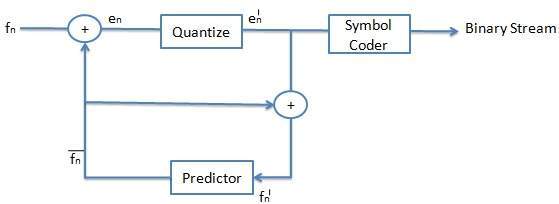
We observed the following point for this figure
As shown in figure, the predictor makes use of the reconstructed, quantized signal values f´n.
The quantizer can be uniform or non-uniform. For any signal, we select the size of quantization steps so that they correspond to the range (maximum and minimum) of the signal.
Codewords for quantized error value e´n are produced using entropy coding (for example Huffman coding). Therefore, the box labeled symbol coder in the figure simply means entropy coding.
The prediction value f¯n is based on previous values of f´n to form the prediction. Therefore we need memory (or buffer) for predictor.
The quantization noise (fn-f´n) is equal to the quantization effect on the error term, en-e´n.
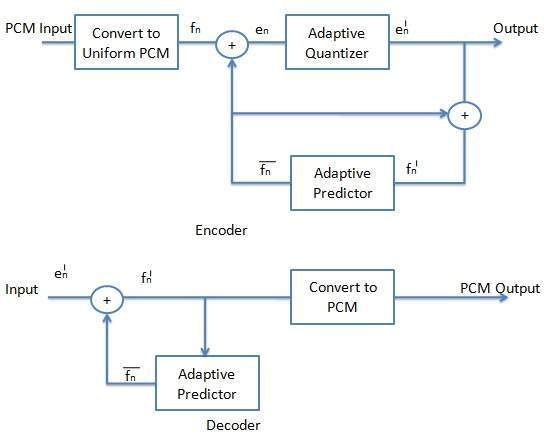
ADPCM (Adaptive DPCM)
DPCM coder has two components, namely the quantizer and the predictor. In Adaptive Differential Pulse Code Modulation (ADPCM), the quantizer and predictor are adaptive. This means that they change to match the characteristics of the speech (or audio) being coded.
ADPCM adapts the quantizer step size to suit the input. In DPCM, step size can be changed along with decision boundaries, using a non uniform quantizer. There are two ways to do this
Forward Adaptive Quantization - Properties of the input signal are used.
Backward Adaptive Quantizationor - Properties of quantized output are used. If errors become too large, choose non-uniform quantizer.
Choose the predictor with forward or backward adaptation to make predictor coefficients adaptive which is also known as Adaptive Predictive Coding (APC). As you know that the predictor is usually a linear function of previous reconstructed quantized value f´n. The number of previous values used is called the order of the predictor. For example, if we use X previous values, we need X coefficients ai, i=1, 2,........, X in predictor. Therefore,
However, we find a different situation, if we try to change the prediction coefficients which multiply previous quantized values to make a complicated set of equations to solve for these cofficients. Figure shows a schematic diagram for the ADPCM encoder and decoder.