Introduction to the Tidyverse

The R package collection known as tidyverse was created with the goal of collaborating and handling data effectively. The Tidyverse package is open-source and constantly improved by the data science community. A data scientist must have a fundamental understanding of every package included under the tidyverse umbrella. All eight packages—purr, ggplot2, dplyr, tidyr, stringr, tibble, readr, and forcats —will be covered in depth.

Tidyverse Packages

Tidyverse groups several packages in R. It consists of the following packages −

Installing Tidyverse

Before moving further, we need to install the tidyverse package in R. You can install this package by using the following command in CRAN −

install.packages("tidyverse")

All the tidyverse packages mentioned above are installed. No need to install these packages separately.

Importing the tidyverse

To import the tidyverse into your R script, you can use the library() function and pass in the tidyverse package as an argument −

library("tidyverse")

Reading Data in the Tidyverse

The “readr” package in R allows us to read from and write into different file formats with the help of functions that start with read% and write%. These functions work very fast and deal smoothly with problematic header names.

These functions are listed below −

Example

Let us see an example illustrating the working of read_csv() function in R −

# Import library
library("tidyverse")

# Import a CSV file
myFile <- read_csv("https://people.sc.fsu.edu/~jburkardt/data/csv/addresses.csv")

# Print the file
myFile

Output

  John                      Doe        `120 jefferson st.`    River…¹  NJ     `08075`
  <chr>                     <chr>      <chr>                  <chr>    <chr>  <chr>  
1 "Jack"                    McGinnis   "220 hobo Av."         Phila    PA     09119  
2 "John "Da Man""           Repici     "120 Jefferson St."    Rivers…  NJ     08075  
3 "Stephen"                 Tyler      "7452 Terrace "At t…   SomeTo…  SD     91234  
4  NA                       Blankman   NA                     SomeTo…  SD     00298  
5 "Joan "the bone", Anne"   Jet        "9th, at Terrace plc"  Desert…  CO     00123  

Data Wrangling in the Tidyverse

dplyr package

The dplyr package allows us to deal with tabular data efficiently. It provides us with verb functions like select() which is used to extract particular columns based on some conditions passed as start_with() or contains() function.

Example

Consider the following program that illustrates the working of these functions −

library(dplyr)
	
# Create a data frame
dataframe <- data.frame( Name = c("Bhuwanesh", "Anil", "Jai", "Naveen"),
   Physics = c(98, 87, 91, 94),
   Chemistry = c(93, 84, 93, 87),
   Mathematics = c(91, 86, 92, 83) )
# Create a data frame
print(dataframe)

Output

       Name Physics Chemistry Mathematics
1 Bhuwanesh      98        93          91
2      Anil      87        84          86
3       Jai      91        93          92
4    Naveen      94        87          83

Print only "Ph" data using the starts_with() function −

library(dplyr)

# Create a data frame
dataframe <- data.frame( Name = c("Bhuwanesh", "Anil", "Jai", "Naveen"),
Physics = c(98, 87, 91, 94),
Chemistry = c(93, 84, 93, 87),
Mathematics = c(91, 86, 92, 83) )
print(select(dataframe, starts_with("Ph")))

Output

  Physics
1      98
2      87
3      91
4      94

Let’s print everything that contains "mist" −

library(dplyr)

# Create a data frame
dataframe <- data.frame( Name = c("Bhuwanesh", "Anil", "Jai", "Naveen"),
Physics = c(98, 87, 91, 94),
Chemistry = c(93, 84, 93, 87),
Mathematics = c(91, 86, 92, 83) )
print(select(dataframe, contains("mist")))

Output

  Chemistry
1        93
2        84
3        93
4        87

As you can see in the output, column names that start with “Ph” and contain “mist” have been extracted.

summary() function

This function produces the summary of a dataset.

print(summary(iris))

Output

  Sepal.Length    Sepal.Width     Petal.Length    Petal.Width   
 Min.   :4.300   Min.   :2.000   Min.   :1.000   Min.   :0.100  
 1st Qu.:5.100   1st Qu.:2.800   1st Qu.:1.600   1st Qu.:0.300  
 Median :5.800   Median :3.000   Median :4.350   Median :1.300  
 Mean   :5.843   Mean   :3.057   Mean   :3.758   Mean   :1.199  
 3rd Qu.:6.400   3rd Qu.:3.300   3rd Qu.:5.100   3rd Qu.:1.800  
 Max.   :7.900   Max.   :4.400   Max.   :6.900   Max.   :2.500  
       Species  
 setosa    :50  
 versicolor:50  
 virginica :50  

The summary() function has produced the summary of the iris model.

filter() function

This function is used to pick data that fulfill specific criteria. For example, consider the following program that shows data in which mathematics marks lie between 90 and 93 −

Example

library(dplyr)

# Create dataframe
dataframe <- data.frame( Name = c("Bhuwanesh", "Anil", "Jai", "Naveen"),
Physics = c(98, 87, 91, 94),
Chemistry = c(93, 84, 93, 87),
Mathematics = c(91, 86, 92, 83) )

# Display
print(dataframe %>% filter(Mathematics > 90 & Mathematics < 94))

Output

       Name Physics Chemistry Mathematics
1 Bhuwanesh      98        93          91
2       Jai      91        93          92

arrange() function

This function is used to arrange the dataset on the basis of a specific column. For example, consider the following program that displays the dataset based on sorted order of physics marks −

Example

library(dplyr)

dataframe <- data.frame( Name = c("Bhuwanesh", "Anil", "Jai", "Naveen"),
Physics = c(98, 87, 91, 94),
Chemistry = c(93, 84, 93, 87),
Mathematics = c(91, 86, 92, 83) )

# Display the data
print(arrange(dataframe, Physics))

Output

       Name Physics Chemistry Mathematics
1      Anil      87        84          86
2       Jai      91        93          92
3    Naveen      94        87          83
4 Bhuwanesh      98        93          91

rename() function

This function is used to rename a column in the dataframe. The first argument corresponds to the new name and the second argument after the equal sign corresponds to the old name. For example, consider the following program that renames the Chemistry column to CHEMISTRY −

Example

library(dplyr)

dataframe <- data.frame( Name = c("Bhuwanesh", "Anil", "Jai", "Naveen"),
Physics = c(98, 87, 91, 94),
Chemistry = c(93, 84, 93, 87),
Mathematics = c(91, 86, 92, 83) )

# Display the dataset
# after renaming a column
print(rename(dataframe, CHEMISTRY = Chemistry))

Output

       Name Physics CHEMISTRY Mathematics
1 Bhuwanesh      98        93          91
2      Anil      87        84          86
3       Jai      91        93          92
4    Naveen      94        87          83

Data Visualization in the Tidyverse

ggplot2 package

The ggplot2 package is an open-source package specially used for data visualization. This is a powerful package designed by Hardley Wickham. This package provides us with various functions. One important function is ggplot(). This function displays the data visualization of a dataset

Example

Consider the following program −

library(ggplot2)

# Plot the data visualization
ggplot(iris, 
aes(x = Sepal.Length, y = Sepal.Width, col = Petal.Length)
) + geom_point()

Output

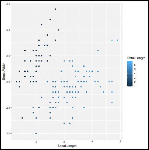
As you can see in the output, the ggplot() function has plotted its visualization.

Function Programming with purrr package

The purrr package is used to achieve functional programming in R. The purrr package provides us map_() family functions, using which we can achieve functional programming to get the same outcome as for and while loops.

Let us discuss the map() function in it. This is the most fundamental function. It accepts a vector and a function as parameters and then calls the function for each element in the vector.

Example

Consider the following program −

library("purrr")

myVector <- c(8, 3, 7, 2, 11, 20)

addByThree <- function(x) + 3

print(map(myVector, addByThree))

Output

[[1]]
[1] 3

[[2]]
[1] 3

[[3]]
[1] 3

[[4]]
[1] 3

[[5]]
[1] 3

[[6]]
[1] 3

As you can see in the above output, a list is produced after adding three to all the elements of the given vector.

String Manipulation with stringr package

The Stringr package is used for string manipulation in R. It provides functions that start with string%. Its most used functions are str_replace() and str_length(). The str_replace() function replaces a pattern or string with another string. Let us consider the following program that illustrates the working of the str_replace() function −

Example

library("stringr")

# Create a list of strings
myList <- c("tutorialspoint", "pointer", "pointable")

# Replace the string equal to "point"
# with “Point”
print(str_replace(myList, "point", "Point"))

Output

[1] "tutorialsPoint" "Pointer"        "Pointable"     

As you can see in the output, the strings containing “point” have been replaced with “Point”.

Example

Let’s consider another example

library("stringr")

myString = "Bhuwanesh Nainwal"

# Replace if string starts with "Bhuwanesh"
print(str_replace(myString, "^Bhuwanesh", "Harshit"))

# Replace if string ends with "Nainwal"
print(str_replace(myString, "Nainwal$", ""))

str_length(myString)

Output

[1] "Harshit Nainwal"
[1] "Bhuwanesh "
17

As you can see in the output, the string that starts with “Bhuwanesh” has been replaced by “Harshit” and the string that ends with “Nainwal” has been replaced with “”.

The str_length() function is used to replace a pattern or string with another string.

Let us consider the following program that illustrates the working of the str_length() function −

Example

library("stringr")
myList <- c("tutorialspoint", "pointer", "pointable")
print(str_length(myList))

Output

[1] 14  7  9

Conclusion

In this tutorial, we discussed the universe of packages, the tidyverse. We discussed how these packages work and illustrated them. This tutorial has definitely helped you to enhance your knowledge in the field of data science.