How to lock column width in pivot table?

In this article, the user will understand how to lock column width in the pivot table. Pivot tables make it easier to explore and analyze large amounts of data by providing a flexible and interactive way to manipulate and present the information in a concise and meaningful format. It enables users to extract insights by summarizing and aggregating data based on different criteria or dimensions.

This article contains a simple example to brief steps by using which the user can lock the column width of the pivot table column. This tutorial will disable the autofit feature of the pivot table.

Example 1: To Lock column width of the pivot table, by disabling the auto-width property

Step 1

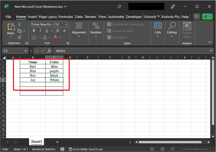
To understand the process of locking the column width of the pivot table, the user first needs to develop a pivot table from the respective table, and then use steps to lock the width of the pivot table. In the below given table, will be using two columns. The first column contains the username, and the second column contains the color name.

Step 2

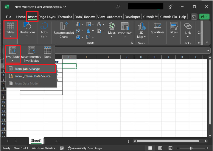
To develop the pivot table, go to the Insert tab, then under the “Tables” section, go to the “Pivot Table” option, and choose the first option for “From Table/Range” as highlighted below −

Step 3

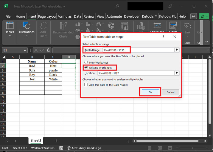
The above step will display an option for “Pivot Table from table/range”. In the Table/Range” dialog box, select the range specified. After that click on the “Existing Worksheet’ option, and in the location label, set the range of data where the user needs to place the pivot table.

Step 4

The above step will display a “Pivot Table Fields” dialog box. This dialog box contains a name for all the columns. In the rows section drag the data value for the name. and in the values column, drag the data value for the count of color.

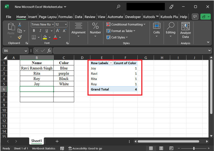
Step 5

The above step will ultimately create a pivot table, as shown below −

Step 6

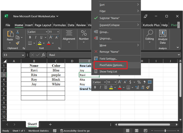
Right click on any cell of the row label, and select the option for “Pivot Table Options”. For proper reference, consider the below-given snapshot −

Step 7

The above step will display a “Pivot Table Options” dialog box. Open the “Layout & Format” option and untick the option for “Autofit column widths on update”. Finally, click on the “OK” button. consider below given image for proper reference −

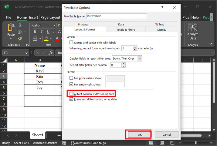
Step 8

Before this step, if any cell value of the name column increases its size, then the pivot table will automatically modify the width of the column. But, after completing the above steps, the automatic size, adjustment becomes disabled. For more clarification, let’s increase the cell data. For this case, will modify the value of the B2 cell, by increasing the size of data present in the cell.

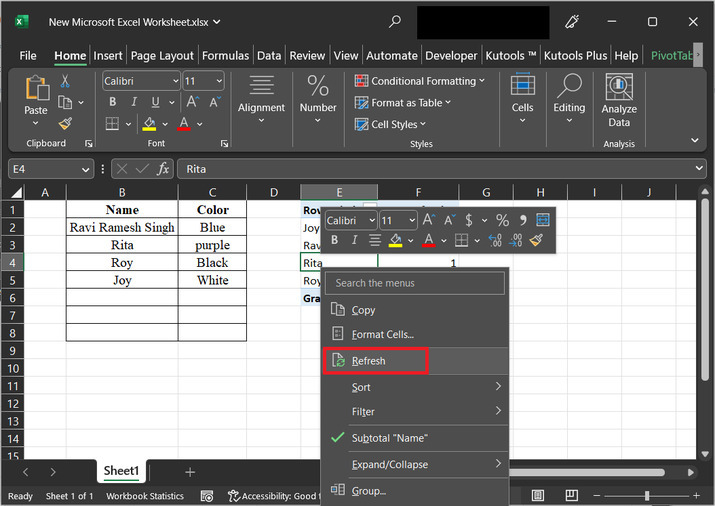
Step 9

Right-click on any cell of the pivot table, this will open a list of menu options. From the visible option list, select an option for “Refresh”. This step will allow the user to refresh the data and display the updated fields in the pivot table. As here the data of B2 cell is updated. So, after using the “Refresh” button, the data will appear again in the Consider the image depicted below for reference:

Step 10

The above step will disable the automatically adjustable property. Due, to this the complete modified name of ravi will not be displayed in the pivot table. But, if user will perform the same task without disabling the required property then the size of column in pivot table, will seems to be changing automatically.

Conclusion

In this article, the user will learn the process of locking the column width of the pivot table, by disabling a property feature. The step-by-step explanation is demonstrated in the example for more clarity and to enhance the user’s knowledge.