How to Hide Error Values in Pivot Table?

In the article, the user will Hide the error values in the pivot table by using the PivotTable Option function. The source data typically contains one or more blank heading cells, which causes the pivot table error "field name is not valid" to show. Each column's heading value is necessary to make a pivot table. There might be some incorrect values in the pivot tables when you make them in Excel. Now, however, it's time to cover up these errors or substitute them with readable text.

Example 1: To hide error values in pivot table in Excel by using the pivot table options

Step 1

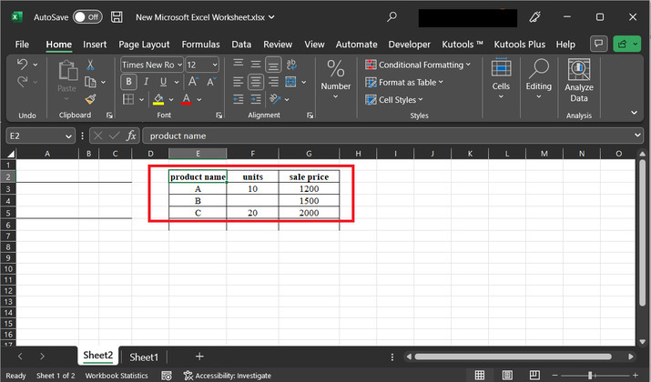
To hide the error values in the pivot table, first, let’s understand the process of generating the required pivot table, and after that will hide the error value, that occurs due to empty data cells.

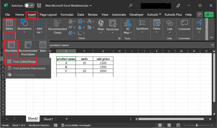
Step 2

In this step, will create a pivot table. To do so, go to the “Insert” tab, and after that go to the “Tables” section, and select the option “PivotTable”. From the available list of options, choose first option for “From Table/Range”. Consider below highlighted image for reference:

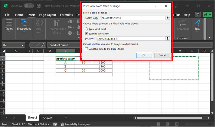
Step 3

The above step will display the “PivotTable from table or range” dialog as shown below. Under the “Table/Range” label select the already provided table. After that select the radio button with the option “Existing Worksheet”. Under the location label, select the location where the user wants to place the pivot table. Consider the below-provided image for proper specifications:

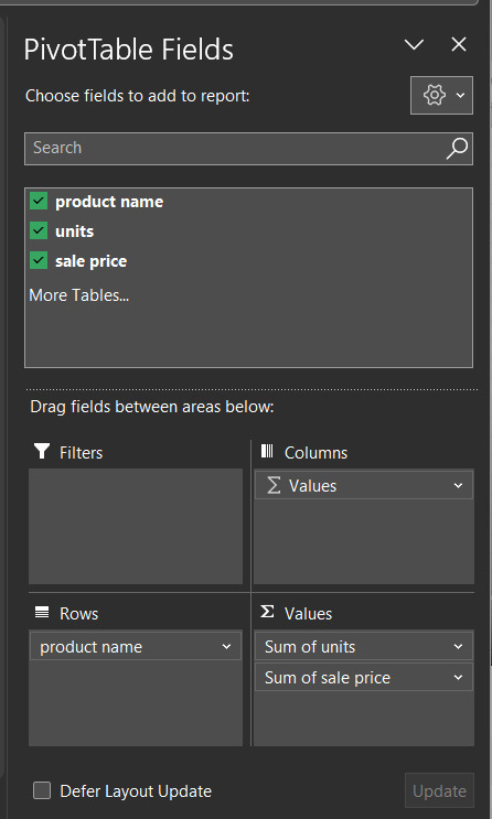
Step 4

The pivot table will display the option, as provided below. First tick option for all the provided row labels. Under the rows option, drag data for “product name”. then under the values header, select “Sum of units”, and “Sum of the sale price”.

Step 5

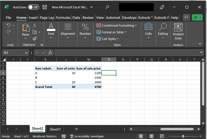
This will display a pivot table to the provided location, with above-mentioned specifications:

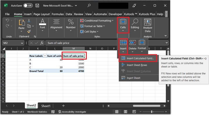
Step 6

After that select the column header for the “Sum of sale price”. Go to the “Home” tab and select the option for “cells”. Then select the option “Insert Calculated Fields”.

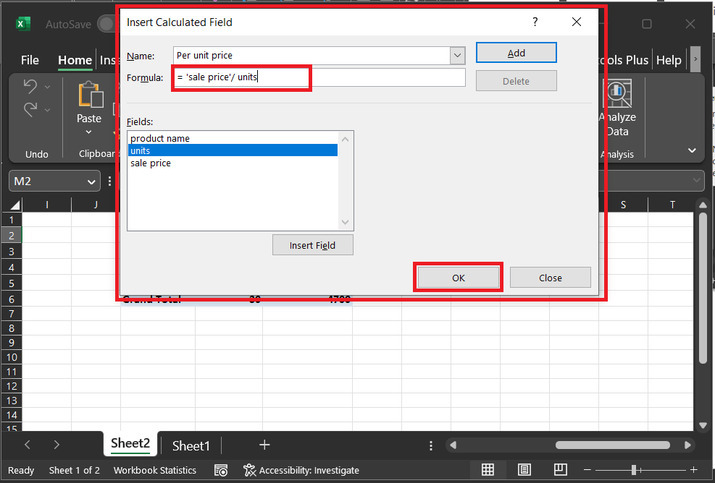
Step 5

The above step will display a dialog box for “Insert Calculated Field”. Under the name label write “Per unit price”, and in the formula bar, write the formula to calculate per unit price as “sale price/ units”. Finally, click on the “OK” button.

Step 6

This will modify the column as given below:

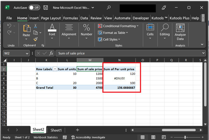
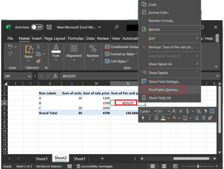
The above image contains an error message for “#DIV/0”, due to division by 0, or an empty cell.

Step 7

Right click on the error message and choose the option for “PivotTable Options”.

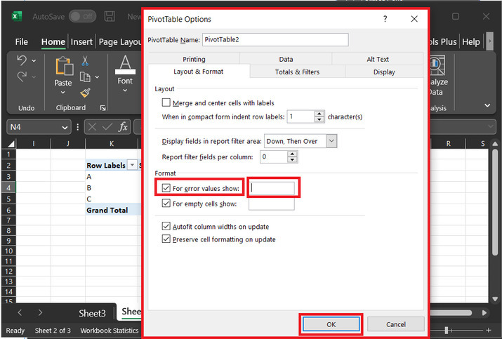
Step 8

This will display a dialog box named PivotTable Options. In the appeared dialog box, go to the “Layout & Format” option tab, tick the option for “For error values show”, and in the front input label type a space. This step will assign a space value to all error containing cells in the pivot table. Finally, click on the “OK” button.

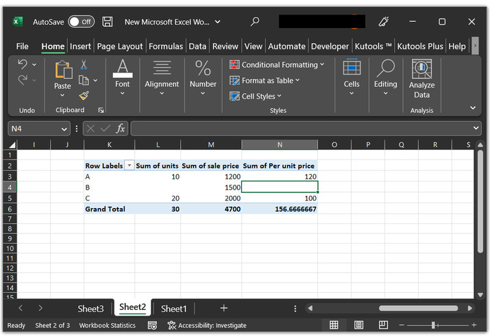
Step 9

Now, the error message will be automatically removed as shown in below image. Pivot table cell with error message is now become empty. As, in the previous step, an empty value is set for the available error cells.

Conclusion

All the above-provided steps are detailed, accurate, and precise. After the successful completion of the above article, the user will be able to hide the error values from a pivot table. The above-guided step is the simplest way to hide the possible error values.