How to go to the specific rows in a worksheet?

An Excel spreadsheet is a combination of rows and columns. Rows are the horizontal lines, on the other hand, groups are the vertical column of the worksheet. This article contains two examples. The first example is based on the use of a name box, and the second example is based on the use of a go-to dialog box. Both examples will guide the user about the process to move to any required cell and location. This example will make the provided cell location active for user editing. Users can write and use the cell according to their requirements.

Example 1: To go to a specific row in the worksheet by using the name box option

Step 1

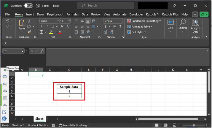
To understand the technique go to the specific row in the worksheet. Consider the below-given worksheet. This worksheet contains data from the D4 to D6 rows.

Step 2

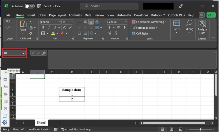
After that go to the “Name box”. This name box contains the current reference of the cell. If the user wants to switch to any specific row, then simply go to the “Name Box” and type your desired location. For example, in this case, the user needs to go to the “B1” cell. So, simply type B1 into the name box, cell as done in the below-given image −

Step 3

This will simply move the cursor to the B1 cell. Users can do whatever is required to do with the B1 cell. This is the simplest and easiest way to move to the desired cell.

Example 2: To go to a specific row in the worksheet by using the Go To dialog box

Step 1

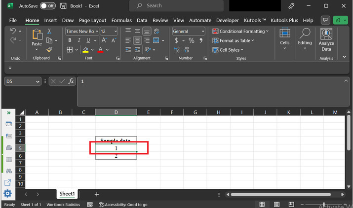
Consider the same worksheet, again. The image snapshot for the sheet is given below −

Step 2

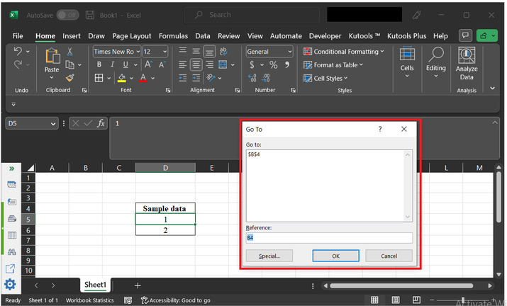
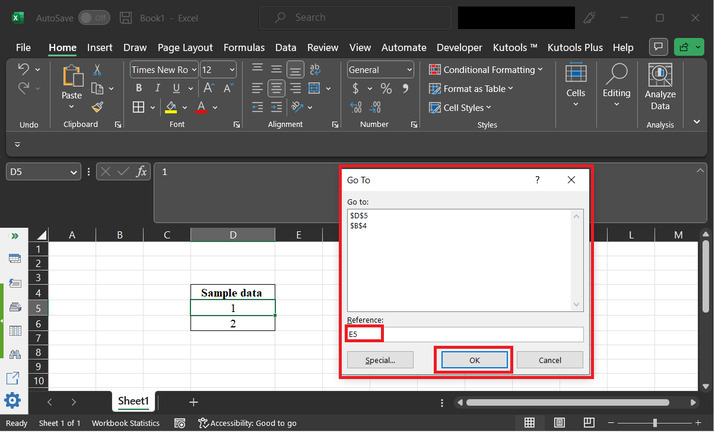
In this example, we will use the go-to option to go to the required cell. Select the “Ctrl+G” keys. This will open a “Go To” dialog box, as specified below. This dialog box contains the previous movement as the option.

Step 3

If the user wants to go to any other cell, then simply go to the “Reference” label, type a valid cell name “E5”, and simply click on the “OK” button, available at the bottom of the Go To dialog box. The options listed in the Go to section such as “D5”, and “B3” are previous active cell locations. Users can click on these value references directly if want to go to any previously provided cell reference. Else “new” cell location can be provided inside the “Reference” label as described above. Consider the below-given image for proper reference −

Step 4

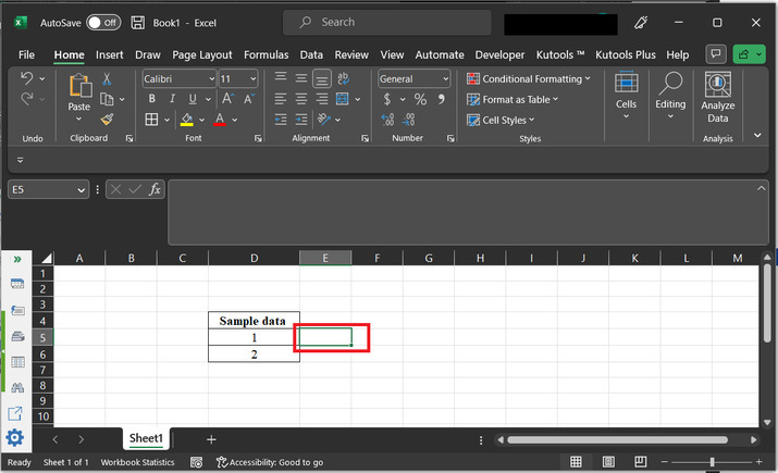
After clicking on the “OK” option. The spreadsheet cell E4 automatically seems to be active for editing. Users can use the active cell for any processing. Refer to the below-given snapshot for a proper explanation.

Conclusion

In this article, two examples are depicted to understand how the users switch to a particular row in a worksheet. Both the provided examples are easy to use and generate effective and efficient results. Using the example more efficiently is based on the learning skills of the learner. If learned effectively understand the methodology, then using both the ways is easy, and accurate.