How to get the max/min of visible cells only in Excel?

Maximum values simply mean the highest data value, and minimum data value contains the least available data values. In this article, the user will learn two ways such as by using the subtotal method to calculate the max and min values, and another possible way is by using kutool to perform the same task. Please understand that both features are already provided by the Excel application software and the user only requires to use the available option, to achieve the possible results.

Example 1: To obtain the maximum and minimum value from the visible cell in Excel by using the SUBTOTAL function:

Step 1:

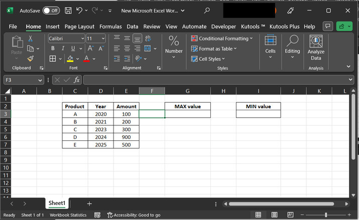
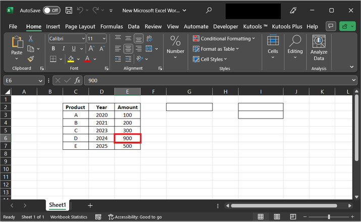
Open the worksheet, and create the same data, as specified below. The provided table contains three columns, the first column contains a name for the product, the second column contains the year, and the third option shows the amount of data. From the provided data table, users need to evaluate the maximum and minimum data values.

Step 2:

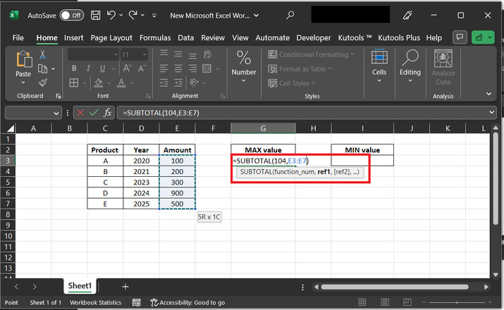
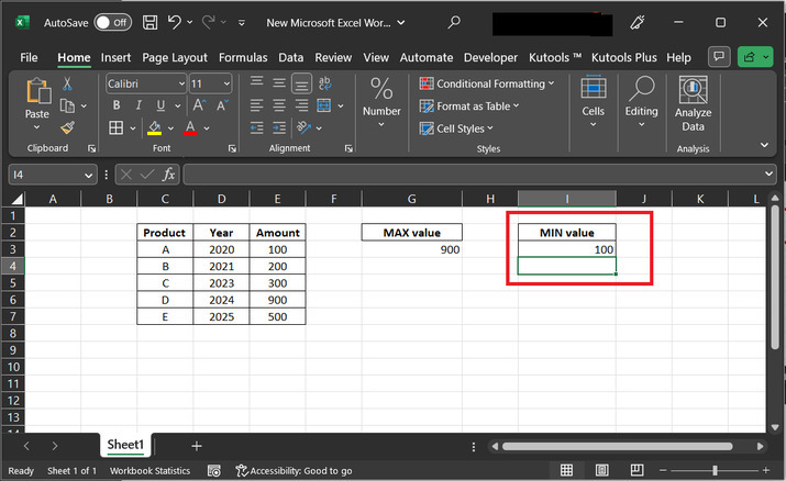
Firstly, will try to evaluate the max value. To do so, first, go to the G2 cell, and type the header for “MAX value”. After that go to the cell G3, and type “=SUBTOTAL(104,E3:E7)”. Consider the below-provided image for reference −

The explanation for the formula:

The Excel function SUBTOTAL is used to calculate a subtotal for a range of cells in a list or table, based on the specified function number. The function number determines the type of calculation that will be performed on the range of cells.

In this case, the function number being used is 104. This represents that the calculation belongs to the sum of the range. The range of cells being summed is specified as E3:E7. Therefore, the SUBTOTAL function will calculate the sum of the values in cells E3 through E7.

It is important to note that the SUBTOTAL function includes only visible cells in the range. If any cells in the range are hidden by a filter or other means, they will be excluded from the calculation. Additionally, the SUBTOTAL function is often used in combination with other Excel functions, such as FILTER or SORT, to create more complex calculations and analyses.

Step 3:

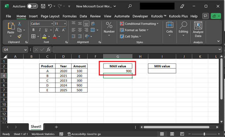
Press the “Enter” key. This will display 100 to the G3 cell as 100 is the minimum value provided within the E column.

Step 4:

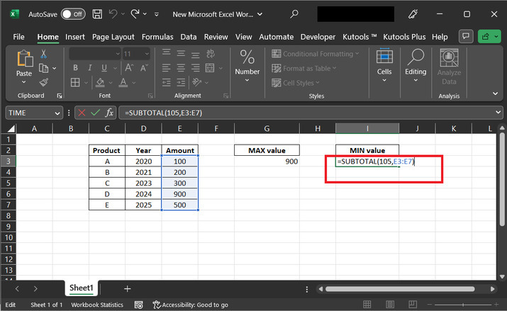
Now, continue the same process to evaluate the minimum value. Go to the I2, cell to define a header for the “MIN” value. After that go to the I3 cell and type “=SUBTOTAL(105,E3:E7)”.

The explanation for the above-used formula:

In this case, the function number being used is 105. This represents the calculation for the count of numbers in the range. The range of cells being counted is specified as E3:E7. Therefore, the SUBTOTAL function will count the number of cells in the range E3 through E7 that contain numbers.

Example 2: To obtain the maximum and minimum value from the visible cell in Excel by using the Kutools extension −

Step 1:

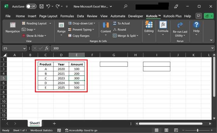
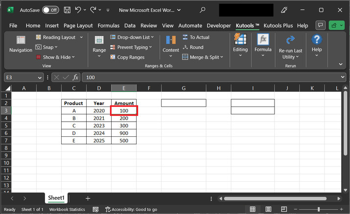
In this example, user will understand the process of using the Kutool to generate both maximum, and minimum numbers. Required snapshot of excel sheet is given below −

Step 2:

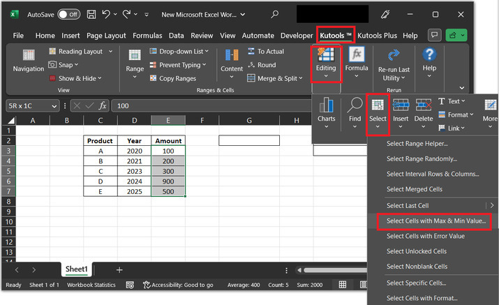
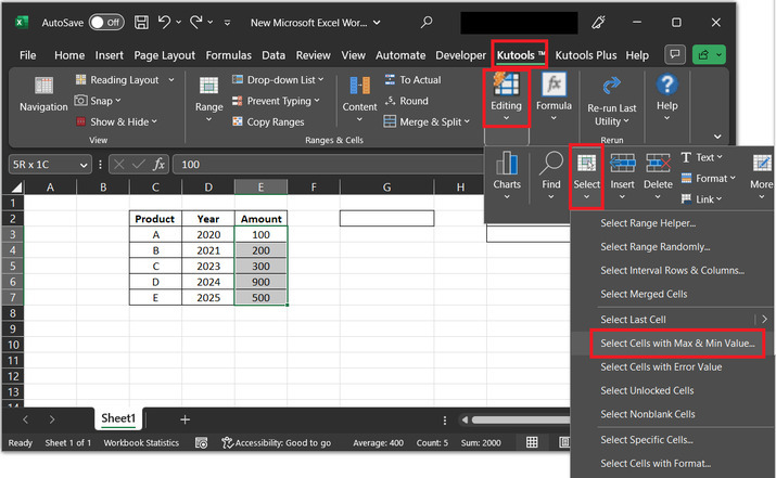
Open the Kutools tab, then go to the “Editing” section, and choose the option for “Select” . Under the “Select” tab, choose the option “Select Cells with Max & Min Value..”. Consider the below-given snapshot to understand the data processing efficiency.

Step 3:

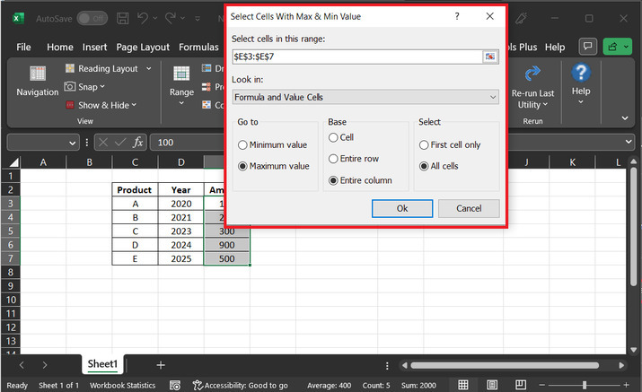
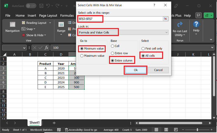
In the select cell in this range label, select the E column, as this column contains values that are required to be filtered. After that in the “Look in −” label set the “Formula and value cells” option. In the “Go to: ” label, select “Minimum value”, in the base label, click on “Entire column”, and in the select label, click on “All cells” . Finally, click on the button “OK”.

Step 4:

This step will automatically move the cursor to the minimum value, as displayed below −

Step 5:

Similarly, to calculate the maximum value. Click on the “kutools” tab and select the “Editing” option. Click on the “Select” tab, and further click on “Select Cells with Max & Min Value”. Consider below provided snapshot for reference −

Step 7:

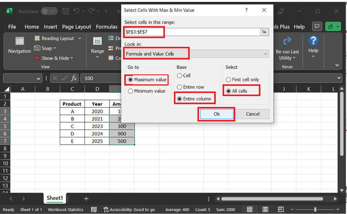
The above step will display a dialog box, with the header “Select Cells with Max & Min value”. Consider the reference image provided below −

Step 8:

In the select cell in this range label, select the E column, as this column contains values that are required to be filtered. After that in the “Look in:” label set the “Formula and Values cells” option. In the “Go to: ” label, select “Maximum value”, in the base label, click on “Entire column”, and in the select label, click on “All cells”. Finally, click on the button “OK”.

Step 9:

This step will automatically move cursor to the maximum value, as displayed below −

Conclusion:

Both the provided example performs the same task, which will evaluate the minimum and maximum data values. The steps-by-steps explanations are demonstrated in both examples. Therefore, after the completion of this article, the user can easily understand the process of generating the maximum and minimum values from the visible cells.