How to display R-squared value on scatterplot with regression model line in R?

The R-squared value is the coefficient of determination, it gives us the percentage or proportion of variation in dependent variable explained by the independent variable. To display this value on the scatterplot with regression model line without taking help from any package, we can use plot function with abline and legend functions.

Consider the below data frame −

Example

 Live Demo

set.seed(1234)
x<-rnorm(20,1,0.096)
y<-rnorm(20,2,0.06)
df<-data.frame(x,y)
df

Output

         x          y
1    0.8841217    2.008045
2    1.0266332    1.970559
3    1.1041064    1.973567
4    0.7748130    2.027575
5    1.0411960    1.958377
6    1.0485814    1.913108
7    0.9448250    2.034485
8    0.9475233    1.938581
9    0.9458126    1.999092
10    0.9145564    1.943843
11    0.9541895    2.066138
12    0.9041549    1.971464
13    0.9254796    1.957434
14    1.0061880    1.969925
15    1.0921114    1.902254
16    0.9894126    1.929943
17    0.9509431    1.869198
18    0.9125252    1.919540
19    0.9196315    1.982342
20    1.2319202    1.972046

Creating the regression model to predict y from x −

Model<-lm(y~x,data=df)
summary(Model)

Call −

lm(formula = y ~ x, data = df)
Residuals:
Min 1Q Median 3Q Max
-0.09955 -0.03138 0.00522 0.02981 0.09783

Coefficients −

Estimate Std. Error t value Pr(>|t|)
(Intercept) 2.0971 0.1084 19.349 1.7e-13 ***
x -0.1350 0.1105 -1.221 0.238 ---
Signif. codes: 0 ‘***’ 0.001 ‘**’ 0.01 ‘*’ 0.05 ‘.’ 0.1 ‘ ’ 1
Residual standard error: 0.04689 on 18 degrees of freedom
Multiple R-squared: 0.07649, Adjusted R-squared: 0.02519
F-statistic: 1.491 on 1 and 18 DF, p-value: 0.2378

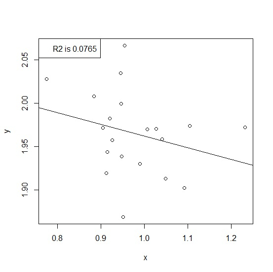
Creating the scatterplot with R-squared value on the plot −

plot(x,y)
abline(Model) legend("topleft",legend=paste("R2 is", format(summary(Model)$r.squared,digits=3)))

Output

Nizamuddin Siddiqui

Updated on: 08-Oct-2020

6K+ Views

Kickstart Your Career

Get certified by completing the course

Get Started