How To Check Or Find If Value Exists In Another Column?

When working with a large array of cells, manually cross-checking if a specific cell value is repeated in another column in the spreadsheet can be difficult and lead to skewed results. Fortunately, there are several options in Microsoft Excel that allow you to do this quickly and efficiently.

In a few simple steps in this tutorial, we demonstrate how to use the Excel functions like VLOOKUP and MATCH to cheack if a value from one column exists in any other column in a worksheet.

Method 1

Finding If Value Exists In Another Column Using VLOOKUP Function

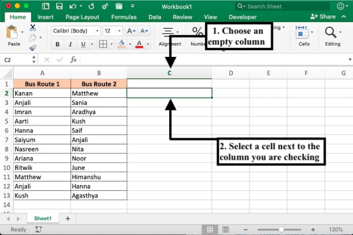
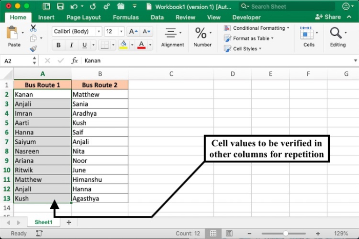
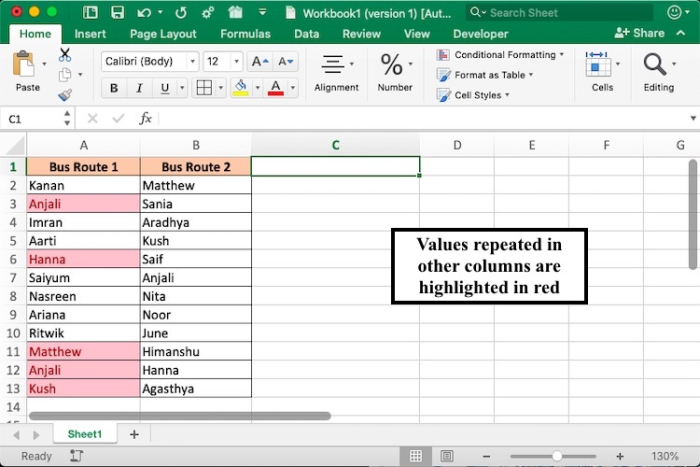
As shown in the example spreadsheet, two columns contain the bus routes and the names of the passengers, and one cannot be present on both routes. To rectify this error, we use the VLOOKUP function to check if names in Column A are not being repeated in Column B.

Step 1 − To verify a value repeated in another column, find an empty cell next to the columns being checked. In this case, we select cell C2.

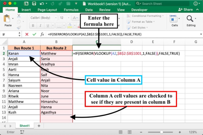
Step 2 − Type in the following formula with VLOOKUP function in the active cell.

Formula to check whether a cell value is being repeated in another column −

=IF(ISERROR(VLOOKUP(A2,$B$2:$B$1001,1,FALSE)),FALSE,TRUE)

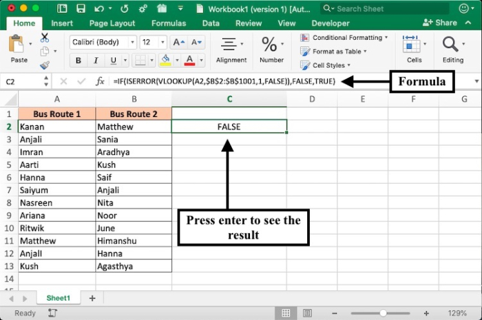
Step 3 − Press the Enter key to see the result.

Step 4 − To replicate the function on the rest of the values of column A, select and drag down the green coloured square box in the bottom right corner of the formula cell.

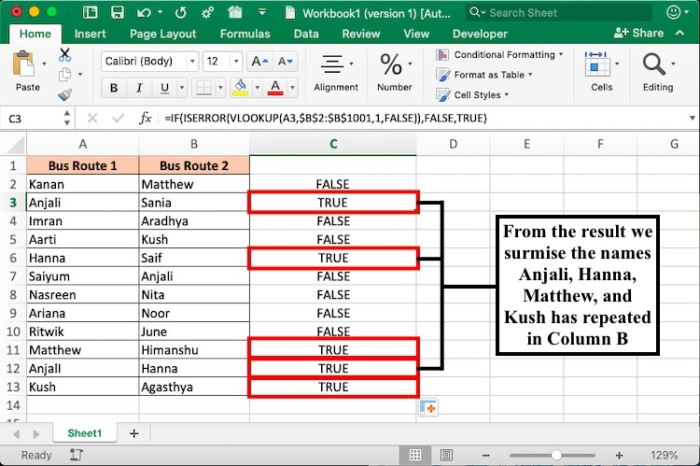
The VLOOKUP is a premade function in MS Excel which searches values across the mentioned columns in the spreadsheet. From the result of the function, we see the names Anjali, Hanna, Matthew, and Kush are repeated in Column B.

Method 2

Finding If Value Exists In Another Column Using MATCH Function with Conditional Formatting

Using this method, you can identify the repeated values in another column and highlight them for visual clarity. It is done using the Conditional Formatting tool, which allows the user to format a cell or range of cells based on the specified formula value.

Step 1 − Select the cells in Column A that should be checked for duplicate values in Column B.

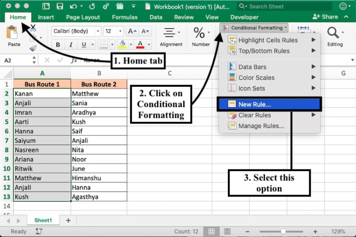
Step 2 − Navigate to the “Home” tab and click on the “Conditional formatting” option. From the dropdown menu, select “New Formatting Rule”.

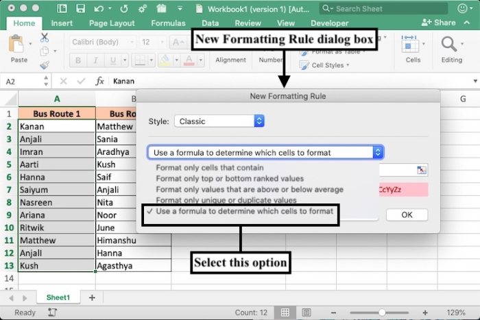
Step 3 − In the “New Formatting Rule” dialog box, select the option “Use a formula to determine which cells to format”.

Step 4 − Enter the formula in the box in the New Formatting Rule dialog box. You can also choose any colour to your preference to highlight the repeated value from the “Format with” dropdown menu.

Formula to find which values of Column A are being repeated in Column B using conditional formatting −

=MATCH(A2,$B$2:$B$13,0)

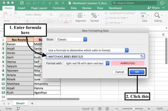
Click on “Okay” to see the results.

Conclusion

The VLOOKUP and the MATCH function help users to find if a specific cell value exists in another column. While in method 1, you get the result in a text value, whereas in method 2, using the conditional formatting feature along with the function gives a clearer visual representation of such values.