- TensorFlow - Home
- TensorFlow - Introduction
- TensorFlow - Installation
- Understanding Artificial Intelligence
- Mathematical Foundations
- Machine Learning & Deep Learning
- TensorFlow - Basics
- Convolutional Neural Networks
- Recurrent Neural Networks
- TensorBoard Visualization
- TensorFlow - Word Embedding
- Single Layer Perceptron
- TensorFlow - Linear Regression
- TFLearn and its installation
- CNN and RNN Difference
- TensorFlow - Keras
- TensorFlow - Distributed Computing
- TensorFlow - Exporting
- Multi-Layer Perceptron Learning
- Hidden Layers of Perceptron
- TensorFlow - Optimizers
- TensorFlow - XOR Implementation
- Gradient Descent Optimization
- TensorFlow - Forming Graphs
- Image Recognition using TensorFlow
- Recommendations for Neural Network Training
TensorFlow - Linear Regression
In this chapter, we will focus on the basic example of linear regression implementation using TensorFlow. Logistic regression or linear regression is a supervised machine learning approach for the classification of order discrete categories. Our goal in this chapter is to build a model by which a user can predict the relationship between predictor variables and one or more independent variables.
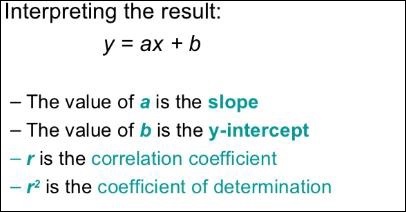
The relationship between these two variables is cons −idered linear. If y is the dependent variable and x is considered as the independent variable, then the linear regression relationship of two variables will look like the following equation −
Y = Ax+b
We will design an algorithm for linear regression. This will allow us to understand the following two important concepts −
- Cost Function
- Gradient descent algorithms
The schematic representation of linear regression is mentioned below −
The graphical view of the equation of linear regression is mentioned below −
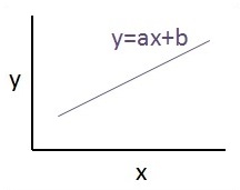
Steps to design an algorithm for linear regression
We will now learn about the steps that help in designing an algorithm for linear regression.
Step 1
It is important to import the necessary modules for plotting the linear regression module. We start importing the Python library NumPy and Matplotlib.
import numpy as np
import matplotlib.pyplot as plt
Step 2
Define the number of coefficients necessary for logistic regression.
number_of_points = 500
x_point = []
y_point = []
a = 0.22
b = 0.78
Step 3
Iterate the variables for generating 300 random points around the regression equation −
Y = 0.22x+0.78
for i in range(number_of_points):
   x = np.random.normal(0.0,0.5)
   y = a*x + b +np.random.normal(0.0,0.1) x_point.append([x])
   y_point.append([y])
Step 4
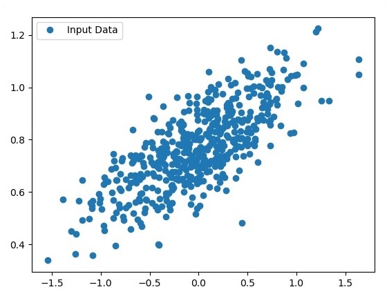
View the generated points using Matplotlib.
fplt.plot(x_point,y_point, 'o', label = 'Input Data') plt.legend() plt.show()
The complete code for logistic regression is as follows −
import numpy as np
import matplotlib.pyplot as plt

number_of_points = 500
x_point = []
y_point = []
a = 0.22
b = 0.78

for i in range(number_of_points):
   x = np.random.normal(0.0,0.5)
   y = a*x + b +np.random.normal(0.0,0.1) x_point.append([x])
   y_point.append([y])

plt.plot(x_point,y_point, 'o', label = 'Input Data') plt.legend()
plt.show()
The number of points which is taken as input is considered as input data.