
Article Categories
- All Categories
-
 Data Structure
-
 Networking
-
 RDBMS
RDBMS
-
 Operating System
-
 Java
Java
-
 MS Excel
-
 iOS
iOS
-
 HTML
HTML
-
 CSS
CSS
-
 Android
-
 Python
-
 C Programming
-
 C++
C++
-
 C#
C#
-
 MongoDB
-
 MySQL
MySQL
-
 Javascript
-
 PHP
PHP
-
 Economics & Finance
Breadth-first Search is a special case of Uniform-cost search in ML
In this article we are going to learn about how Breadth-first search is a specific case of Uniform-Cost search in ML. Regardless of who is doing it (humans or AI), they must consider every scenario that might result from changing the starting state to the objective state (if one exists), as well as all conceivable outcomes. The same is true for AI systems, which employ a variety of search methods depending on the desired state (if it exists).
What is Breadth-first search?
It is an AI search method that explores a tree breadthwise to find the objective. The most common approach is the Breadth-First Search Algorithm (BFS). BFS is a graph traversal technique in which you start at a source node and work your way through the graph, studying nodes that are closely linked to the source node. Then, in BFS traversal, you must go to the next-level neighbor nodes.
According to the BFS, you must explore the graph in a breadthwise direction ?
- Begin by moving horizontally and visiting all of the nodes in the current layer.
- Continue to the next tier.
When doing a breadth-first search, a queue data structure is used to store the node and mark it as "visited" when it has marked all of the nearby vertices that are directly connected to it. According to the First In First Out (FIFO) principle, the queue views the neighbors of each node in the order in which it adds them, beginning with the node that was placed first.
Advantages
Whenever a solution becomes available, BFS will provide it.
In the event that there are many solutions to a certain issue, BFS will provide the one with the fewest steps and the lowest cost.
Disadvantages
As each level of the tree must be stored in memory before expanding to the following level, a lot of memory is needed.
If the answer is located distant from the root node, BFS requires a lot of time.
Pseudocode
<div class="code-mirror  language-python" contenteditable="plaintext-only" spellcheck="false" style="outline: none; overflow-wrap: break-word; overflow-y: auto; white-space: pre-wrap;">Bredth_First_Serach<span class="token punctuation">(</span> G<span class="token punctuation">,</span> A <span class="token punctuation">)</span> <span class="token operator">//</span> G <span class="token keyword">is</span> the graph<span class="token punctuation">,</span> <span class="token keyword">and</span> A <span class="token keyword">is</span> the source node
Let q be the queue
q<span class="token punctuation">.</span>enqueue<span class="token punctuation">(</span> A <span class="token punctuation">)</span> <span class="token operator">//</span> Inserting source node A to the queue
Mark A node <span class="token keyword">as</span> visited<span class="token punctuation">.</span>
While <span class="token punctuation">(</span> q <span class="token keyword">is</span> <span class="token keyword">not</span> empty <span class="token punctuation">)</span>
B <span class="token operator">=</span> q<span class="token punctuation">.</span>dequeue<span class="token punctuation">(</span> <span class="token punctuation">)</span> <span class="token operator">//</span> Removing that vertex <span class="token keyword">from</span> the queue<span class="token punctuation">,</span> which will be
visited by its neighbour
Processing <span class="token builtin">all</span> the neighbours of B
For <span class="token builtin">all</span> neighbours of C of B
C <span class="token keyword">is</span> <span class="token keyword">not</span> visited<span class="token punctuation">,</span> q<span class="token punctuation">.</span> enqueue<span class="token punctuation">(</span> C <span class="token punctuation">)</span> <span class="token operator">//</span>Stores C <span class="token keyword">in</span> q to visit its neighbour
Mark C a visited
</div>
What is Uniform Cost Search?
When the step costs differ yet the target state must be solved optimally, this approach is typically utilized. When this occurs, we employ a uniform cost search to identify the objective as well as the path, which includes the total cost incurred by expanding each node from the root node to the target node. It does not search in depth or breadth; instead, it looks for the next node with the lowest cost. In the instance of a path with the same cost, let's take lexicographical order into account.
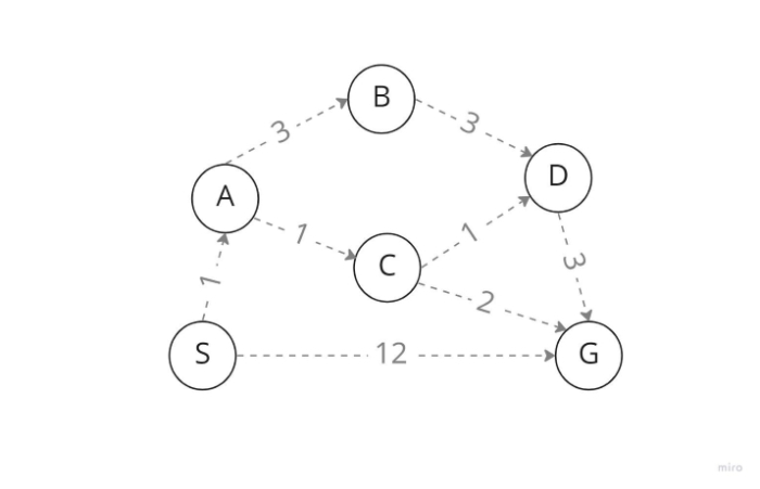
Think of S as the start node and G as the goal state in the diagram above. We search for a node to expand from node S, and our options are nodes A and G. However, because this is a uniform cost search, it expands the node with the lowest step cost, making node A the successor rather than our necessary target node G. We examine B and C, A's offspring nodes, from A. Therefore, as node C has the lowest step cost, it traverses through node C. Then, since nodes D and G are successors of C and have low step costs, we expand with D as well.
Finally, by using UFS Algorithm, we obtain the target state D since D has just one kid G, which is the conditional goal state we need. Instead of traveling directly to G, where the cost is 12 and 6<<12, if we have traveled this route, our total path cost from S to G is only 6, even after passing through several nodes (in terms of step cost). But not every situation may be suitable for this.
Advantages
The least expensive path is selected at each state, making uniform cost search the best option.
Disadvantages
It is primarily concerned with path cost and gives no thought to how many steps are involved in the search process. As a result, this algorithm could become trapped in an endless cycle.
Pseudocode
<div class="code-mirror  language-python" contenteditable="plaintext-only" spellcheck="false" style="outline: none; overflow-wrap: break-word; overflow-y: auto; white-space: pre-wrap;">function UCS<span class="token punctuation">(</span>Graph<span class="token punctuation">,</span> start<span class="token punctuation">,</span> target<span class="token punctuation">)</span><span class="token punctuation">:</span>
   Add the starting node to the opened <span class="token builtin">list</span><span class="token punctuation">.</span> The node has
   has zero distance value <span class="token keyword">from</span> itself
   <span class="token keyword">while</span> <span class="token boolean">True</span><span class="token punctuation">:</span>
      <span class="token keyword">if</span> opened <span class="token keyword">is</span> empty<span class="token punctuation">:</span>
         <span class="token keyword">break</span> <span class="token comment"># No solution found</span>
      selecte_node <span class="token operator">=</span> remove <span class="token keyword">from</span> opened <span class="token builtin">list</span><span class="token punctuation">,</span> the node <span class="token keyword">with</span>
         the minimun distance value
      <span class="token keyword">if</span> selected_node <span class="token operator">==</span> target<span class="token punctuation">:</span>
         calculate path
         <span class="token keyword">return</span> path
      add selected_node to closed <span class="token builtin">list</span>
      new_nodes <span class="token operator">=</span> get the children of selected_node
      <span class="token keyword">if</span> the selected node has children<span class="token punctuation">:</span>
         <span class="token keyword">for</span> each child <span class="token keyword">in</span> children<span class="token punctuation">:</span>
            calculate the distance value of child
            <span class="token keyword">if</span> child <span class="token keyword">not</span> <span class="token keyword">in</span> closed <span class="token keyword">and</span> opened lists<span class="token punctuation">:</span>
               child<span class="token punctuation">.</span>parent <span class="token operator">=</span> selected_node
               add the child to opened <span class="token builtin">list</span>
      <span class="token keyword">else</span> <span class="token keyword">if</span> child <span class="token keyword">in</span> opened <span class="token builtin">list</span><span class="token punctuation">:</span>
         <span class="token keyword">if</span> the distance value of child <span class="token keyword">is</span> lower than
            the corresponding node <span class="token keyword">in</span> opened <span class="token builtin">list</span><span class="token punctuation">:</span>
               child<span class="token punctuation">.</span>parent <span class="token operator">=</span> selected_node
               add the child to opened <span class="token builtin">list</span>
</div>
Driving Uniform Cost Search from Breadth-First Search
UCS enhances Breadth-First Search by adding three changes.
To begin, it employs a priority queue as its border. It arranges the frontier nodes according to g, the cost of the journey from the start node to the border nodes. When selecting a node for expansion, UCS chooses the one with the smallest value of g, i.e. the one with the lowest cost, from the frontier.
However, just because we've added a node to the frontier doesn't imply we know what the best path to the node's state costs. If we extend a node v and discover that the path from v to its neighbor u is less expensive than g(w), where w is a frontier node representing the same state as u, we should remove w from the frontier and replace it with u. The second change is the queue updating step.
The third is to perform the aim test after we have expanded the node, rather than when we have placed it in the frontier. We might return a suboptimal path to the goal if we verify the nodes before placing them in the queue. Why? Because UCS has the ability to identify a better path later in its execution.
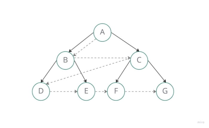
Consider the following example of a suboptimal path returned by Breadth-First Search. If we stop searching immediately after expanding Start and seeing that the goal node Goal is its neighbor, we will miss the ideal path that goes via A.
Conclusion
The Uninformed Search techniques for searching are a multifunctional strategy that combines the capability of unguided search with raw force. Because they lack knowledge about state space and target issues, the algorithms of this technique can be used to solve a wide range of computer science problems.

3K+ Views
