How To Create A Dynamic Chart Title In Excel?

Excel is a powerful tool that allows users to create visually appealing charts to represent data. However, the title of the chart is just as important as the data itself. A dynamic chart title in Excel can make a huge difference in the way your chart is perceived and can convey more information than a static title. In this tutorial, we will guide you step-by-step on how to create a dynamic chart title in Excel. Here, we can use the Name box to complete the task. So let us see a simple process to know how you can create a dynamic chart title in Excel. With a dynamic chart title, you can easily customize the title to reflect changes in your data, which makes your chart more informative and professional-looking. Whether you're a beginner or an experienced user, this tutorial will help you create dynamic chart titles quickly and easily.

Create A Dynamic Chart Title

In this tutorial, we will see a simple method for knowing how you can create a dynamic chart title in Excel. We can simply complete the task using the name box.

Step 1

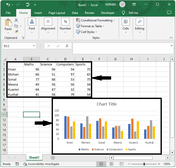
Consider an Excel sheet where you have a chart similar to the below image.

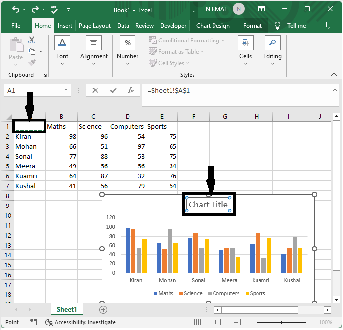
First, double-click on the chart title, click on an empty cell (in our case, cell A1), and click enter.

Chart tittle > Empty cell > Enter.

Step 2

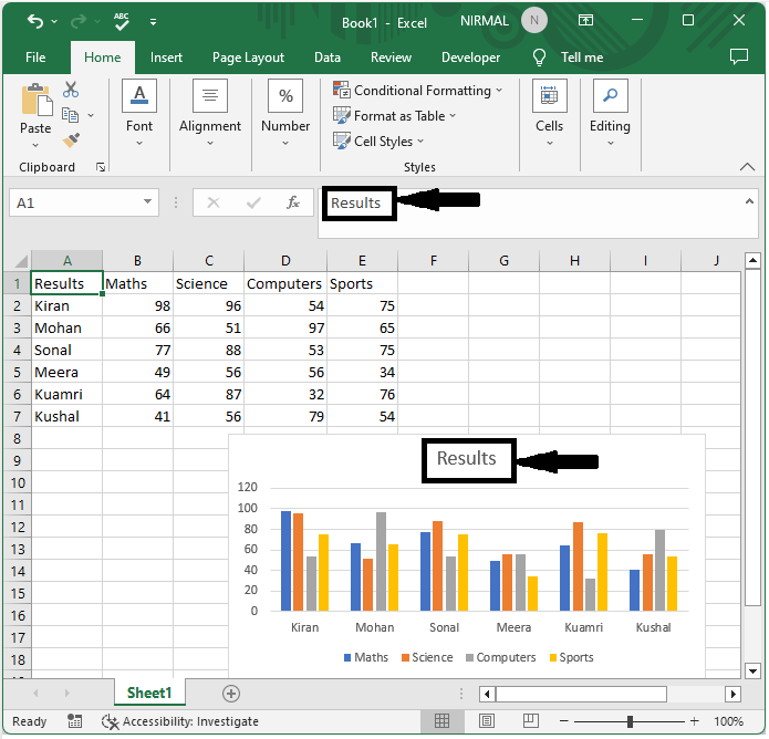
From now on, we can see that the data entered in cell A1 will be displayed as a chart title.

Conclusion

In this tutorial, we have used a simple example to demonstrate how you can create a dynamic chart title in Excel to highlight a particular set of data. Finally, we can conclude that we can complete our task just by using the name box.