- Apache MXNet - Home
- Apache MXNet - Introduction
- Apache MXNet - Installing MXNet
- Apache MXNet - Toolkits and Ecosystem
- Apache MXNet - System Architecture
- Apache MXNet - System Components
- Apache MXNet - Unified Operator API
- Apache MXNet - Distributed Training
- Apache MXNet - Python Packages
- Apache MXNet - NDArray
- Apache MXNet - Gluon
- Apache MXNet - KVStore and Visualization
- Apache MXNet - Python API ndarray
- Apache MXNet - Python API gluon
- Apache MXNet - Python API autograd and initializer
- Apache MXNet - Python API Symbol
- Apache MXNet - Python API Module
- Apache MXNet Useful Resources
- Apache MXNet - Quick Guide
- Apache MXNet - Useful Resources
- Apache MXNet - Discussion
Apache MXNet - Quick Guide
Apache MXNet - Introduction
This chapter highlights the features of Apache MXNet and talks about the latest version of this deep learning software framework.
What is MXNet?
Apache MXNet is a powerful open-source deep learning software framework instrument helping developers build, train, and deploy Deep Learning models. Past few years, from healthcare to transportation to manufacturing and, in fact, in every aspect of our daily life, the impact of deep learning has been widespread. Nowadays, deep learning is sought by companies to solve some hard problems like Face recognition, object detection, Optical Character Recognition (OCR), Speech Recognition, and Machine Translation.
Thats the reason Apache MXNet is supported by:
Some big companies like Intel, Baidu, Microsoft, Wolfram Research, etc.
Public cloud providers including Amazon Web Services (AWS), and Microsoft Azure
Some big research institutes like Carnegie Mellon, MIT, the University of Washington, and the Hong Kong University of Science & Technology.
Why Apache MXNet?
There are various deep learning platforms like Torch7, Caffe, Theano, TensorFlow, Keras, Microsoft Cognitive Toolkit, etc. existed then you might wonder why Apache MXNet? Lets check out some of the reasons behind it:
Apache MXNet solves one of the biggest issues of existing deep learning platforms. The issue is that in order to use deep learning platforms one must need to learn another system for a different programming flavor.
With the help of Apache MXNet developers can exploit the full capabilities of GPUs as well as cloud computing.
Apache MXNet can accelerate any numerical computation and places a special emphasis on speeding up the development and deployment of large-scale DNN (deep neural networks).
It provides the users the capabilities of both imperative and symbolic programming.
Various Features
If you are looking for a flexible deep learning library to quickly develop cutting-edge deep learning research or a robust platform to push production workload, your search ends at Apache MXNet. It is because of the following features of it:
Distributed Training
Whether it is multi-gpu or multi-host training with near-linear scaling efficiency, Apache MXNet allows developers to make most out of their hardware. MXNet also support integration with Horovod, which is an open source distributed deep learning framework created at Uber.
For this integration, following are some of the common distributed APIs defined in Horovod:
horovod.broadcast()
horovod.allgather()
horovod.allgather()
In this regard, MXNet offer us the following capabilities:
Device Placement − With the help of MXNet we can easily specify each data structure (DS).
Automatic Differentiation − Apache MXNet automates the differentiation i.e. derivative calculations.
Multi-GPU training − MXNet allows us to achieve scaling efficiency with number of available GPUs.
Optimized Predefined Layers − We can code our own layers in MXNet as well as the optimized the predefined layers for speed also.
Hybridization
Apache MXNet provides its users a hybrid front-end. With the help of the Gluon Python API it can bridge the gap between its imperative and symbolic capabilities. It can be done by calling its hybridize functionality.
Faster Computation
The linear operations like tens or hundreds of matrix multiplications are the computational bottleneck for deep neural nets. To solve this bottleneck MXNet provides −
Optimized numerical computation for GPUs
Optimized numerical computation for distributed ecosystems
Automation of common workflows with the help of which the standard NN can be expressed briefly.
Language Bindings
MXNet has deep integration into high-level languages like Python and R. It also provides support for other programming languages such as-
Scala
Julia
Clojure
Java
C/C++
Perl
We do not need to learn any new programming language instead MXNet, combined with hybridization feature, allows an exceptionally smooth transition from Python to deployment in the programming language of our choice.
Latest version MXNet 1.6.0
Apache Software Foundation (ASF) has released the stable version 1.6.0 of Apache MXNet on 21st February 2020 under Apache License 2.0. This is the last MXNet release to support Python 2 as MXNet community voted to no longer support Python 2 in further releases. Let us check out some of the new features this release brings for its users.
NumPy-Compatible interface
Due to its flexibility and generality, NumPy has been widely used by Machine Learning practitioners, scientists, and students. But as we know that, these days hardware accelerators like Graphical Processing Units (GPUs) have become increasingly assimilated into various Machine Learning (ML) toolkits, the NumPy users, to take advantage of the speed of GPUs, need to switch to new frameworks with different syntax.
With MXNet 1.6.0, Apache MXNet is moving toward a NumPy-compatible programming experience. The new interface provides equivalent usability as well as expressiveness to the practitioners familiar with NumPy syntax. Along with that MXNet 1.6.0 also enables the existing Numpy system to utilize hardware accelerators like GPUs to speed-up large-scale computations.
Integration with Apache TVM
Apache TVM, an open-source end-to-end deep learning compiler stack for hardware-backends such as CPUs, GPUs, and specialized accelerators, aims to fill the gap between the productivity-focused deep-learning frameworks and performance-oriented hardware backends. With the latest release MXNet 1.6.0, users can leverage Apache(incubating) TVM to implement high-performance operator kernels in Python programming language. Two main advantages of this new feature are following −
Simplifies the former C++ based development process.
Enables sharing the same implementation across multiple hardware backend such as CPUs, GPUs, etc.
Improvements on existing features
Apart from the above listed features of MXNet 1.6.0, it also provides some improvements over the existing features. The improvements are as follows −
Grouping element-wise operation for GPU
As we know the performance of element-wise operations is memory-bandwidth and that is the reason, chaining such operations may reduce overall performance. Apache MXNet 1.6.0 does element-wise operation fusion, that actually generates just-in-time fused operations as and when possible. Such element-wise operation fusion also reduces storage needs and improve overall performance.
Simplifying common expressions
MXNet 1.6.0 eliminates the redundant expressions and simplify the common expressions. Such enhancement also improves memory usage and total execution time.
Optimizations
MXNet 1.6.0 also provides various optimizations to existing features & operators, which are as follows:
Automatic Mixed Precision
Gluon Fit API
MKL-DNN
Large tensor Support
TensorRT integration
Higher-order gradient support
Operators
Operator performance profiler
ONNX import/export
Improvements to Gluon APIs
Improvements to Symbol APIs
More than 100 bug fixes
Apache MXNet - Installing MXNet
To get started with MXNet, the first thing we need to do, is to install it on our computer. Apache MXNet works on pretty much all the platforms available, including Windows, Mac, and Linux.
Linux OS
We can install MXNet on Linux OS in the following ways −
Graphical Processing Unit (GPU)
Here, we will use various methods namely Pip, Docker, and Source to install MXNet when we are using GPU for processing −
By using Pip method
You can use the following command to install MXNet on your Linus OS −
pip install mxnet
Apache MXNet also offers MKL pip packages, which are much faster when running on intel hardware. Here for example mxnet-cu101mkl means that −
The package is built with CUDA/cuDNN
The package is MKL-DNN enabled
The CUDA version is 10.1
For other option you can also refer to https://pypi.org/project/mxnet/.
By using Docker
You can find the docker images with MXNet at DockerHub, which is available at https://hub.docker.com/u/mxnet Let us check out the steps below to install MXNet by using Docker with GPU −
Step 1− First, by following the docker installation instructions which are available at https://docs.docker.com/engine/install/ubuntu/. We need to install Docker on our machine.
Step 2− To enable the usage of GPUs from the docker containers, next we need to install nvidia-docker-plugin. You can follow the installation instructions given at https://github.com/NVIDIA/nvidia-docker/wiki.
Step 3− By using the following command, you can pull the MXNet docker image −
$ sudo docker pull mxnet/python:gpu
Now in order to see if mxnet/python docker image pull was successful, we can list docker images as follows −
$ sudo docker images
For the fastest inference speeds with MXNet, it is recommended to use the latest MXNet with Intel MKL-DNN. Check the commands below −
$ sudo docker pull mxnet/python:1.3.0_cpu_mkl
$ sudo docker images
From source
To build the MXNet shared library from source with GPU, first we need to set up the environment for CUDA and cuDNN as follows−
Download and install CUDA toolkit, here CUDA 9.2 is recommended.
Next download cuDNN 7.1.4.
Now we need to unzip the file. It is also required to change to the cuDNN root directory. Also move the header and libraries to local CUDA Toolkit folder as follows −
tar xvzf cudnn-9.2-linux-x64-v7.1
sudo cp -P cuda/include/cudnn.h /usr/local/cuda/include
sudo cp -P cuda/lib64/libcudnn* /usr/local/cuda/lib64
sudo chmod a+r /usr/local/cuda/include/cudnn.h /usr/local/cuda/lib64/libcudnn*
sudo ldconfig
After setting up the environment for CUDA and cuDNN, follow the steps below to build the MXNet shared library from source −
Step 1− First, we need to install the prerequisite packages. These dependencies are required on Ubuntu version 16.04 or later.
sudo apt-get update
sudo apt-get install -y build-essential git ninja-build ccache libopenblas-dev
libopencv-dev cmake
Step 2− In this step, we will download MXNet source and configure. First let us clone the repository by using following command−
git clone recursive https://github.com/apache/incubator-mxnet.git mxnet
cd mxnet
cp config/linux_gpu.cmake #for build with CUDA
Step 3− By using the following commands, you can build MXNet core shared library−
rm -rf build
mkdir -p build && cd build
cmake -GNinja ..
cmake --build .
Two important points regarding the above step is as follows−
If you want to build the Debug version, then specify the as follows−
cmake -DCMAKE_BUILD_TYPE=Debug -GNinja ..
In order to set the number of parallel compilation jobs, specify the following −
cmake --build . --parallel N
Once you successfully build MXNet core shared library, in the build folder in your MXNet project root, you will find libmxnet.so which is required to install language bindings(optional).
Central Processing Unit (CPU)
Here, we will use various methods namely Pip, Docker, and Source to install MXNet when we are using CPU for processing −
By using Pip method
You can use the following command to install MXNet on your Linus OS−
pip install mxnet
Apache MXNet also offers MKL-DNN enabled pip packages which are much faster, when running on intel hardware.
pip install mxnet-mkl
By using Docker
You can find the docker images with MXNet at DockerHub, which is available at https://hub.docker.com/u/mxnet. Let us check out the steps below to install MXNet by using Docker with CPU −
Step 1− First, by following the docker installation instructions which are available at https://docs.docker.com/engine/install/ubuntu/. We need to install Docker on our machine.
Step 2− By using the following command, you can pull the MXNet docker image:
$ sudo docker pull mxnet/python
Now, in order to see if mxnet/python docker image pull was successful, we can list docker images as follows −
$ sudo docker images
For the fastest inference speeds with MXNet, it is recommended to use the latest MXNet with Intel MKL-DNN.
Check the commands below −
$ sudo docker pull mxnet/python:1.3.0_cpu_mkl
$ sudo docker images
From source
To build the MXNet shared library from source with CPU, follow the steps below −
Step 1− First, we need to install the prerequisite packages. These dependencies are required on Ubuntu version 16.04 or later.
sudo apt-get update

sudo apt-get install -y build-essential git ninja-build ccache libopenblas-dev libopencv-dev cmake
Step 2− In this step we will download MXNet source and configure. First let us clone the repository by using following command:
git clone recursive https://github.com/apache/incubator-mxnet.git mxnet

cd mxnet
cp config/linux.cmake config.cmake
Step 3− By using the following commands, you can build MXNet core shared library:
rm -rf build
mkdir -p build && cd build
cmake -GNinja ..
cmake --build .
Two important points regarding the above step is as follows−
If you want to build the Debug version, then specify the as follows:
cmake -DCMAKE_BUILD_TYPE=Debug -GNinja ..
In order to set the number of parallel compilation jobs, specify the following−
cmake --build . --parallel N
Once you successfully build MXNet core shared library, in the build folder in your MXNet project root, you will find libmxnet.so, which is required to install language bindings(optional).
MacOS
We can install MXNet on MacOS in the following ways−
Graphical Processing Unit (GPU)
If you plan to build MXNet on MacOS with GPU, then there is NO Pip and Docker method available. The only method in this case is to build it from source.
From source
To build the MXNet shared library from source with GPU, first we need to set up the environment for CUDA and cuDNN. You need to follow the NVIDIA CUDA Installation Guide which is available at https://docs.nvidia.com and cuDNN Installation Guide, which is available at https://docs.nvidia.com/deeplearning/cudnn/installation/latest/linux.html for mac OS.
Please note that in 2019 CUDA stopped supporting macOS. In fact, future versions of CUDA may also not support macOS.
Once you set up the environment for CUDA and cuDNN, follow the steps given below to install MXNet from source on OS X (Mac)−
Step 1− As we need some dependencies on OS x, First, we need to install the prerequisite packages.
xcode-select -install #Install OS X Developer Tools

/usr/bin/ruby -e "$(curl -fsSL https://raw.githubusercontent.com/Homebrew/install/master/install)" #Install Homebrew

brew install cmake ninja ccache opencv # Install dependencies
We can also build MXNet without OpenCV as opencv is an optional dependency.
Step 2− In this step we will download MXNet source and configure. First let us clone the repository by using following command−
git clone -recursive https://github.com/apache/incubator-mxnet.git mxnet

cd mxnet
cp config/linux.cmake config.cmake
For a GPU-enabled, it is necessary to install the CUDA dependencies first because when one tries to build a GPU-enabled build on a machine without GPU, MXNet build cannot autodetect your GPU architecture. In such cases MXNet will target all available GPU architectures.
Step 3− By using the following commands, you can build MXNet core shared library−
rm -rf build
mkdir -p build && cd build
cmake -GNinja ..
cmake --build .
Two important points regarding the above step is as follows−
If you want to build the Debug version, then specify the as follows−
cmake -DCMAKE_BUILD_TYPE=Debug -GNinja ..
In order to set the number of parallel compilation jobs, specify the following:
cmake --build . --parallel N
Once you successfully build MXNet core shared library, in the build folder in your MXNet project root, you will find libmxnet.dylib, which is required to install language bindings(optional).
Central Processing Unit (CPU)
Here, we will use various methods namely Pip, Docker, and Source to install MXNet when we are using CPU for processing−
By using Pip method
You can use the following command to install MXNet on your Linus OS
pip install mxnet
By using Docker
You can find the docker images with MXNet at DockerHub, which is available at https://hub.docker.com/u/mxnet. Let us check out the steps below to install MXNet by using Docker with CPU−
Step 1− First, by following the docker installation instructions which are available at https://docs.docker.com/docker-for-mac we need to install Docker on our machine.
Step 2− By using the following command, you can pull the MXNet docker image−
$ docker pull mxnet/python
Now in order to see if mxnet/python docker image pull was successful, we can list docker images as follows−
$ docker images
For the fastest inference speeds with MXNet, it is recommended to use the latest MXNet with Intel MKL-DNN. Check the commands below−
$ docker pull mxnet/python:1.3.0_cpu_mkl
$ docker images
From source
Follow the steps given below to install MXNet from source on OS X (Mac)−
Step 1− As we need some dependencies on OS x, first, we need to install the prerequisite packages.
xcode-select -install #Install OS X Developer Tools
/usr/bin/ruby -e "$(curl -fsSL https://raw.githubusercontent.com/Homebrew/install/master/install)" #Install Homebrew
brew install cmake ninja ccache opencv # Install dependencies
We can also build MXNet without OpenCV as opencv is an optional dependency.
Step 2− In this step we will download MXNet source and configure. First, let us clone the repository by using following command−
git clone -recursive https://github.com/apache/incubator-mxnet.git mxnet

cd mxnet

cp config/linux.cmake config.cmake
Step 3− By using the following commands, you can build MXNet core shared library:
rm -rf build
mkdir -p build && cd build
cmake -GNinja ..
cmake --build .
Two important points regarding the above step is as follows−
If you want to build the Debug version, then specify the as follows−
cmake -DCMAKE_BUILD_TYPE=Debug -GNinja ..
In order to set the number of parallel compilation jobs, specify the following−
cmake --build . --parallel N
Once you successfully build MXNet core shared library, in the build folder in your MXNet project root, you will find libmxnet.dylib, which is required to install language bindings(optional).
Windows OS
To install MXNet on Windows, following are the prerequisites−
Minimum System Requirements
Windows 7, 10, Server 2012 R2, or Server 2016
Visual Studio 2015 or 2017 (any type)
Python 2.7 or 3.6
pip
Recommended System Requirements
Windows 10, Server 2012 R2, or Server 2016
Visual Studio 2017
At least one NVIDIA CUDA-enabled GPU
MKL-enabled CPU: Intel Xeon processor, Intel Core processor family, Intel Atom processor, or Intel Xeon Phi processor
Python 2.7 or 3.6
pip
Graphical Processing Unit (GPU)
By using Pip method−
If you plan to build MXNet on Windows with NVIDIA GPUs, there are two options for installing MXNet with CUDA support with a Python package−
Install with CUDA Support
Below are the steps with the help of which, we can setup MXNet with CUDA.
Step 1− First install Microsoft Visual Studio 2017 or Microsoft Visual Studio 2015.
Step 2− Next, download and install NVIDIA CUDA. It is recommended to use CUDA versions 9.2 or 9.0 because some issues with CUDA 9.1 have been identified in the past.
Step 3− Now, download and install NVIDIA_CUDA_DNN.
Step 4− Finally, by using following pip command, install MXNet with CUDA−
pip install mxnet-cu92
Install with CUDA and MKL Support
Below are the steps with the help of which, we can setup MXNet with CUDA and MKL.
Step 1− First install Microsoft Visual Studio 2017 or Microsoft Visual Studio 2015.
Step 2− Next, download and install intel MKL
Step 3− Now, download and install NVIDIA CUDA.
Step 4− Now, download and install NVIDIA_CUDA_DNN.
Step 5− Finally, by using following pip command, install MXNet with MKL.
pip install mxnet-cu92mkl
From source
To build the MXNet core library from source with GPU, we have the following two options−
Option 1− Build with Microsoft Visual Studio 2017
In order to build and install MXNet yourself by using Microsoft Visual Studio 2017, you need the following dependencies.
Install/update Microsoft Visual Studio.
If Microsoft Visual Studio is not already installed on your machine, first download and install it.
It will prompt about installing Git. Install it also.
If Microsoft Visual Studio is already installed on your machine but you want to update it then proceed to the next step to modify your installation. Here you will be given the opportunity to update Microsoft Visual Studio as well.
Follow the instructions for opening the Visual Studio Installer available at https://docs.microsoft.com/en-us to modify Individual components.
In the Visual Studio Installer application, update as required. After that look for and check VC++ 2017 version 15.4 v14.11 toolset and click Modify.
Now by using the following command, change the version of the Microsoft VS2017 to v14.11−
"C:\Program Files (x86)\Microsoft Visual Studio\2017\Community\VC\Auxiliary\Build\vcvars64.bat" -vcvars_ver=14.11
Next, you need to download and install CMake available at https://cmake.org/download/ It is recommended to use CMake v3.12.2 which is available at https://cmake.org/download/ because it is tested with MXNet.
Now, download and run the OpenCV package available at https://sourceforge.net/projects/opencvlibrary/which will unzip several files. It is up to you if you want to place them in another directory or not. Here, we will use the path C:\utils(mkdir C:\utils) as our default path.
Next, we need to set the environment variable OpenCV_DIR to point to the OpenCV build directory that we have just unzipped. For this open command prompt and type set OpenCV_DIR=C:\utils\opencv\build.
One important point is that if you do not have the Intel MKL (Math Kernel Library) installed the you can install it.
Another open source package you can use is OpenBLAS. Here for the further instructions we are assuming that you are using OpenBLAS.
So, Download the OpenBlas package which is available at https://sourceforge.net and unzip the file, rename it to OpenBLAS and put it under C:\utils.
Next, we need to set the environment variable OpenBLAS_HOME to point to the OpenBLAS directory that contains the include and lib directories. For this open command prompt and type set OpenBLAS_HOME=C:\utils\OpenBLAS.
Now, download and install CUDA available at https://developer.nvidia.com. Note that, if you already had CUDA, then installed Microsoft VS2017, you need to reinstall CUDA now, so that you can get the CUDA toolkit components for Microsoft VS2017 integration.
Next, you need to download and install cuDNN.
Next, you need to download and install git which is at https://gitforwindows.org/ also.
Once you have installed all the required dependencies, follow the steps given below to build the MXNet source code−
Step 1− Open command prompt in windows.
Step 2− Now, by using the following command, download the MXNet source code from GitHub:
cd C:\

git clone https://github.com/apache/incubator-mxnet.git --recursive
Step 3− Next, verify the following−
DCUDNN_INCLUDE and DCUDNN_LIBRARY environment variables are pointing to the include folder and cudnn.lib file of your CUDA installed location
C:\incubator-mxnet is the location of the source code you just cloned in the previous step.
Step 4− Next by using the following command, create a build directory and also go to the directory, for example−
mkdir C:\incubator-mxnet\build
cd C:\incubator-mxnet\build
Step 5− Now, by using cmake, compile the MXNet source code as follows−
cmake -G "Visual Studio 15 2017 Win64" -T cuda=9.2,host=x64 -DUSE_CUDA=1 -DUSE_CUDNN=1 -DUSE_NVRTC=1 -DUSE_OPENCV=1 -DUSE_OPENMP=1 -DUSE_BLAS=open -DUSE_LAPACK=1 -DUSE_DIST_KVSTORE=0 -DCUDA_ARCH_LIST=Common -DCUDA_TOOLSET=9.2 -DCUDNN_INCLUDE=C:\cuda\include -DCUDNN_LIBRARY=C:\cuda\lib\x64\cudnn.lib "C:\incubator-mxnet"
Step 6− Once the CMake successfully completed, use the following command to compile the MXNet source code−
msbuild mxnet.sln /p:Configuration=Release;Platform=x64 /maxcpucount
Option 2: Build with Microsoft Visual Studio 2015
In order to build and install MXNet yourself by using Microsoft Visual Studio 2015, you need the following dependencies.
Install/update Microsoft Visual Studio 2015. The minimum requirement to build MXnet from source is of Update 3 of Microsoft Visual Studio 2015. You can use Tools -> Extensions and Updates... | Product Updates menu to upgrade it.
Next, you need to download and install CMake which is available at https://cmake.org/download/. It is recommended to use CMake v3.12.2 which is at https://cmake.org/download/, because it is tested with MXNet.
Now, download and run the OpenCV package available at https://excellmedia.dl.sourceforge.net which will unzip several files. It is up to you, if you want to place them in another directory or not.
Next, we need to set the environment variable OpenCV_DIR to point to the OpenCV build directory that we have just unzipped. For this, open command prompt and type set OpenCV_DIR=C:\opencv\build\x64\vc14\bin.
One important point is that if you do not have the Intel MKL (Math Kernel Library) installed the you can install it.
Another open source package you can use is OpenBLAS. Here for the further instructions we are assuming that you are using OpenBLAS.
So, Download the OpenBLAS package available at https://excellmedia.dl.sourceforge.net and unzip the file, rename it to OpenBLAS and put it under C:\utils.
Next, we need to set the environment variable OpenBLAS_HOME to point to the OpenBLAS directory that contains the include and lib directories. You can find the directory in C:\Program files (x86)\OpenBLAS\
Note that, if you already had CUDA, then installed Microsoft VS2015, you need to reinstall CUDA now so that, you can get the CUDA toolkit components for Microsoft VS2017 integration.
Next, you need to download and install cuDNN.
Now, we need to Set the environment variable CUDACXX to point to the CUDA Compiler(C:\Program Files\NVIDIA GPU Computing Toolkit\CUDA\v9.1\bin\nvcc.exe for example).
Similarly, we also need to set the environment variable CUDNN_ROOT to point to the cuDNN directory that contains the include, lib and bin directories (C:\Downloads\cudnn-9.1-windows7-x64-v7\cuda for example).
Once you have installed all the required dependencies, follow the steps given below to build the MXNet source code−
Step 1− First, download the MXNet source code from GitHub−
cd C:\
git clone https://github.com/apache/incubator-mxnet.git --recursive
Step 2− Next, use CMake to create a Visual Studio in ./build.
Step 3− Now, in Visual Studio, we need to open the solution file,.sln, and compile it. These commands will produce a library called mxnet.dll in the ./build/Release/ or ./build/Debug folder
Step 4− Once the CMake successfully completed, use the following command to compile the MXNet source code
msbuild mxnet.sln /p:Configuration=Release;Platform=x64 /maxcpucount
Central Processing Unit (CPU)
Here, we will use various methods namely Pip, Docker, and Source to install MXNet when we are using CPU for processing−
By using Pip method
If you plan to build MXNet on Windows with CPUs, there are two options for installing MXNet using a Python package−
Install with CPUs
Use the following command to install MXNet with CPU with Python−
pip install mxnet
Install with Intel CPUs
As discussed above, MXNet has experimental support for Intel MKL as well as MKL-DNN. Use the following command to install MXNet with Intel CPU with Python−
pip install mxnet-mkl
By using Docker
You can find the docker images with MXNet at DockerHub, available at https://hub.docker.com/u/mxnet Let us check out the steps below, to install MXNet by using Docker with CPU−
Step 1− First, by following the docker installation instructions which can be read at https://docs.docker.com/docker-for-mac/install. We need to install Docker on our machine.
Step 2− By using the following command, you can pull the MXNet docker image−
$ docker pull mxnet/python
Now in order to see if mxnet/python docker image pull was successful, we can list docker images as follows−
$ docker images
For the fastest inference speeds with MXNet, it is recommended to use the latest MXNet with Intel MKL-DNN.
Check the commands below−
$ docker pull mxnet/python:1.3.0_cpu_mkl
$ docker images
Installing MXNet On Cloud and Devices
This section highlights how to install Apache MXNet on Cloud and on devices. Let us begin by learning about installing MXNet on cloud.
Installing MXNet On Cloud
You can also get Apache MXNet on several cloud providers with Graphical Processing Unit (GPU) support. Two other kind of support you can find are as follows−
- GPU/CPU-hybrid support for use cases like scalable inference.
- Factorial GPU support with AWS Elastic Inference.
Following are cloud providers providing GPU support with different virtual machine for Apache MXNet−
The Alibaba Console
You can create the NVIDIA GPU Cloud Virtual Machine (VM) available at https://docs.nvidia.com/ngc with the Alibaba Console and use Apache MXNet.
Amazon Web Services
It also provides GPU support and gives the following services for Apache MXNet−
Amazon SageMaker
It manages training and deployment of Apache MXNet models.
AWS Deep Learning AMI
It provides preinstalled Conda environment for both Python 2 and Python 3 with Apache MXNet, CUDA, cuDNN, MKL-DNN, and AWS Elastic Inference.
Dynamic Training on AWS
It provides the training for experimental manual EC2 setup as well as for semi-automated CloudFormation setup.
You can use NVIDIA VM available at https://aws.amazon.com with Amazon web services.
Google Cloud Platform
Google is also providing NVIDIA GPU cloud image which is available at https://console.cloud.google.com to work with Apache MXNet.
Microsoft Azure
Microsoft Azure Marketplace is also providing NVIDIA GPU cloud image available at https://azuremarketplace.microsoft.com to work with Apache MXNet.
Oracle Cloud
Oracle is also providing NVIDIA GPU cloud image available at https://docs.cloud.oracle.com to work with Apache MXNet.
Central Processing Unit (CPU)
Apache MXNet works on every cloud providers CPU-only instance. There are various methods to install such as−
Python pip install instructions.
Docker instructions.
Preinstalled option like Amazon Web Services which provides AWS Deep Learning AMI (having preinstalled Conda environment for both Python 2 and Python 3 with MXNet and MKL-DNN).
Installing MXNet on Devices
Let us learn how to install MXNet on devices.
Raspberry Pi
You can also run Apache MXNet on Raspberry Pi 3B devices as MXNet also support Respbian ARM based OS. In order to run MXNet smoothly on the Raspberry Pi3, it is recommended to have a device that has more than 1 GB of RAM and a SD card with at least 4GB of free space.
Following are the ways with the help of which you can build MXNet for the Raspberry Pi and install the Python bindings for the library as well−
Quick installation
The pre-built Python wheel can be used on a Raspberry Pi 3B with Stretch for quick installation. One of the important issues with this method is that, we need to install several dependencies to get Apache MXNet to work.
Docker installation
You can follow the docker installation instructions, which is available at https://docs.docker.com/engine/install/ubuntu/ to install Docker on your machine. For this purpose, we can install and use Community Edition (CE) also.
Native Build (from source)
In order to install MXNet from source, we need to follow the following two steps−
Step 1
Build the shared library from the Apache MXNet C++ source code
To build the shared library on Raspberry version Wheezy and later, we need the following dependencies:
Git− It is required to pull code from GitHub.
Libblas− It is required for linear algebraic operations.
Libopencv− It is required for computer vision related operations. However, it is optional if you would like to save your RAM and Disk Space.
C++ Compiler− It is required to compiles and builds MXNet source code. Following are the supported compilers that supports C++ 11−
G++ (4.8 or later version)
Clang(3.9-6)
Use the following commands to install the above-mentioned dependencies−
sudo apt-get update
sudo apt-get -y install git cmake ninja-build build-essential g++-4.9 c++-4.9 liblapack*
libblas* libopencv*
libopenblas* python3-dev python-dev virtualenv
Next, we need to clone the MXNet source code repository. For this use the following git command in your home directory−
git clone https://github.com/apache/incubator-mxnet.git --recursive

cd incubator-mxnet
Now, with the help of following commands, build the shared library:
mkdir -p build && cd build
cmake \
-DUSE_SSE=OFF \
-DUSE_CUDA=OFF \
-DUSE_OPENCV=ON \
-DUSE_OPENMP=ON \
-DUSE_MKL_IF_AVAILABLE=OFF \
-DUSE_SIGNAL_HANDLER=ON \

-DCMAKE_BUILD_TYPE=Release \
-GNinja ..
ninja -j$(nproc)
Once you execute the above commands, it will start the build process which will take couple of hours to finish. You will get a file named libmxnet.so in the build directory.
Step 2
Install the supported language-specific packages for Apache MXNet
In this step, we will install MXNet Pythin bindings. To do so, we need to run the following command in the MXNet directory−
cd python
pip install --upgrade pip
pip install -e .
Alternatively, with the following command, you can also create a whl package installable with pip−
ci/docker/runtime_functions.sh build_wheel python/ $(realpath build)
NVIDIA Jetson Devices
You can also run Apache MXNet on NVIDIA Jetson Devices, such as TX2 or Nano as MXNet also support the Ubuntu Arch64 based OS. In order to run, MXNet smoothly on the NVIDIA Jetson Devices, it is necessary to have CUDA installed on your Jetson device.
Following are the ways with the help of which you can build MXNet for NVIDIA Jetson devices:
By using a Jetson MXNet pip wheel for Python development
From source
But, before building MXNet from any of the above-mentioned ways, you need to install following dependencies on your Jetson devices−
Python Dependencies
In order to use the Python API, we need the following dependencies−
sudo apt update
sudo apt -y install \
   build-essential \
   git \
   graphviz \
   libatlas-base-dev \
   libopencv-dev \
   python-pip
sudo pip install --upgrade \
   pip \
   setuptools
sudo pip install \
   graphviz==0.8.4 \
   jupyter \
   numpy==1.15.2
Clone the MXNet source code repository
By using the following git command in your home directory, clone the MXNet source code repository−
git clone --recursive https://github.com/apache/incubator-mxnet.git mxnet
Setup environment variables
Add the following in your .profile file in your home directory−
export PATH=/usr/local/cuda/bin:$PATH
export MXNET_HOME=$HOME/mxnet/
export PYTHONPATH=$MXNET_HOME/python:$PYTHONPATH
Now, apply the change immediately with the following command−
source .profile
Configure CUDA
Before configuring CUDA, with nvcc, you need to check what version of CUDA is running−
nvcc --version
Suppose, if more than one CUDA version is installed on your device or computer and you want to switch CUDA versions then, use the following and replace the symbolic link to the version you want−
sudo rm /usr/local/cuda
sudo ln -s /usr/local/cuda-10.0 /usr/local/cuda
The above command will switch to CUDA 10.0, which is preinstalled on NVIDIA Jetson device Nano.
Once you done with the above-mentioned prerequisites, you can now install MXNet on NVIDIA Jetson Devices. So, let us understand the ways with the help of which you can install MXNet−
By using a Jetson MXNet pip wheel for Python development− If you want to use a prepared Python wheel then download the following to your Jetson and run it−
MXNet 1.4.0 (for Python 3) available at https://docs.docker.com
MXNet 1.4.0 (for Python 2) available at https://docs.docker.com
Native Build (from source)
In order to install MXNet from source, we need to follow the following two steps−
Step 1
Build the shared library from the Apache MXNet C++ source code
To build the shared library from the Apache MXNet C++ source code, you can either use Docker method or do it manually−
Docker method
In this method, you first need to install Docker and able to run it without sudo (which is also explained in previous steps). Once done, run the following to execute cross-compilation via Docker−
$MXNET_HOME/ci/build.py -p jetson
Manual
In this method, you need to edit the Makefile (with below command) to install the MXNet with CUDA bindings to leverage the Graphical Processing units (GPU) on NVIDIA Jetson devices:
cp $MXNET_HOME/make/crosscompile.jetson.mk config.mk
After editing the Makefile, you need to edit config.mk file to make some additional changes for the NVIDIA Jetson device.
For this, update the following settings−
Update the CUDA path: USE_CUDA_PATH = /usr/local/cuda
Add -gencode arch=compute-63, code=sm_62 to the CUDA_ARCH setting.
Update the NVCC settings: NVCCFLAGS := -m64
Turn on OpenCV: USE_OPENCV = 1
Now to ensure that the MXNet builds with Pascals hardware level low precision acceleration, we need to edit the Mshadow Makefile as follow−
MSHADOW_CFLAGS += -DMSHADOW_USE_PASCAL=1
Finally, with the help of following command you can build the complete Apache MXNet library−
cd $MXNET_HOME
make -j $(nproc)
Once you execute the above commands, it will start the build process which will take couple of hours to finish. You will get a file named libmxnet.so in the mxnet/lib directory.
Step 2
Install the Apache MXNet Python Bindings
In this step, we will install MXNet Python bindings. To do so we need to run the following command in the MXNet directory−
cd $MXNET_HOME/python
sudo pip install -e .
Once done with above steps, you are now ready to run MXNet on your NVIDIA Jetson devices TX2 or Nano. It can be verified with the following command−
import mxnet
mxnet.__version__
It will return the version number if everything is properly working.
Apache MXNet - Toolkits and Ecosystem
To support the research and development of Deep Learning applications across many fields, Apache MXNet provides us a rich ecosystem of toolkits, libraries and many more. Let us explore them −
ToolKits
Following are some of the most used and important toolkits provided by MXNet −
GluonCV
As name implies GluonCV is a Gluon toolkit for computer vision powered by MXNet. It provides implementation of state-of-the-art DL (Deep Learning) algorithms in computer vision (CV). With the help of GluonCV toolkit engineers, researchers, and students can validate new ideas and learn CV easily.
Given below are some of the features of GluonCV −
It trains scripts for reproducing state-of-the-art results reported in latest research.
More than 170+ high quality pretrained models.
Embrace flexible development pattern.
GluonCV is easy to optimize. We can deploy it without retaining heavy weight DL framework.
It provides carefully designed APIs that greatly lessen the implementation intricacy.
Community support.
Easy to understand implementations.
Following are the supported applications by GluonCV toolkit:
Image Classification
Object Detection
Semantic Segmentation
Instance Segmentation
Pose Estimation
Video Action Recognition
We can install GluonCV by using pip as follows −
pip install --upgrade mxnet gluoncv
GluonNLP
As name implies GluonNLP is a Gluon toolkit for Natural Language Processing (NLP) powered by MXNet. It provides implementation of state-of-the-art DL (Deep Learning) models in NLP.
With the help of GluonNLP toolkit engineers, researchers, and students can build blocks for text data pipelines and models. Based on these models, they can quickly prototype the research ideas and product.
Given below are some of the features of GluonNLP:
It trains scripts for reproducing state-of-the-art results reported in latest research.
Set of pretrained models for common NLP tasks.
It provides carefully designed APIs that greatly lessen the implementation intricacy.
Community support.
It also provides tutorials to help you get started on new NLP tasks.
Following are the NLP tasks we can implement with GluonNLP toolkit −
Word Embedding
Language Model
Machine Translation
Text Classification
Sentiment Analysis
Natural Language Inference
Text Generation
Dependency Parsing
Named Entity Recognition
Intent Classification and Slot Labeling
We can install GluonNLP by using pip as follows −
pip install --upgrade mxnet gluonnlp
GluonTS
As name implies GluonTS is a Gluon toolkit for Probabilistic Time Series Modeling powered by MXNet.
It provides the following features −
State-of-the-art (SOTA) deep learning models ready to be trained.
The utilities for loading as well as iterating over time-series datasets.
Building blocks to define your own model.
With the help of GluonTS toolkit engineers, researchers, and students can train and evaluate any of the built-in models on their own data, quickly experiment with different solutions, and come up with a solution for their time series tasks.
They can also use the provided abstractions and building blocks to create custom time series models, and rapidly benchmark them against baseline algorithms.
We can install GluonTS by using pip as follows −
pip install gluonts
GluonFR
As name implies, it is an Apache MXNet Gluon toolkit for FR (Face Recognition). It provides the following features −
State-of-the-art (SOTA) deep learning models in face recognition.
The implementation of SoftmaxCrossEntropyLoss, ArcLoss, TripletLoss, RingLoss, CosLoss/AMsoftmax, L2-Softmax, A-Softmax, CenterLoss, ContrastiveLoss, and LGM Loss, etc.
In order to install Gluon Face, we need Python 3.5 or later. We also first need to install GluonCV and MXNet first as follows −
pip install gluoncv --pre
pip install mxnet-mkl --pre --upgrade
pip install mxnet-cuXXmkl --pre upgrade # if cuda XX is installed
Once you installed the dependencies, you can use the following command to install GluonFR −
From Source
pip install git+https://github.com/THUFutureLab/gluon-face.git@master
Pip
pip install gluonfr
Ecosystem
Now let us explore MXNets rich libraries, packages, and frameworks −
Coach RL
Coach, a Python Reinforcement Learning (RL) framework created by Intel AI lab. It enables easy experimentation with State-of-the-art RL algorithms. Coach RL supports Apache MXNet as a back end and allows simple integration of new environment to solve.
In order to extend and reuse existing components easily, Coach RL very well decoupled the basic reinforcement learning components such as algorithms, environments, NN architectures, exploration policies.
Following are the agents and supported algorithms for Coach RL framework −
Value Optimization Agents
Deep Q Network (DQN)
Double Deep Q Network (DDQN)
Dueling Q Network
Mixed Monte Carlo (MMC)
Persistent Advantage Learning (PAL)
Categorical Deep Q Network (C51)
Quantile Regression Deep Q Network (QR-DQN)
N-Step Q Learning
Neural Episodic Control (NEC)
Normalized Advantage Functions (NAF)
Rainbow
Policy Optimization Agents
Policy Gradients (PG)
Asynchronous Advantage Actor-Critic (A3C)
Deep Deterministic Policy Gradients (DDPG)
Proximal Policy Optimization (PPO)
Clipped Proximal Policy Optimization (CPPO)
Generalized Advantage Estimation (GAE)
Sample Efficient Actor-Critic with Experience Replay (ACER)
Soft Actor-Critic (SAC)
Twin Delayed Deep Deterministic Policy Gradient (TD3)
General Agents
Direct Future Prediction (DFP)
Imitation Learning Agents
Behavioral Cloning (BC)
Conditional Imitation Learning
Hierarchical Reinforcement Learning Agents
Hierarchical Actor Critic (HAC)
Deep Graph Library
Deep Graph Library (DGL), developed by NYU and AWS teams, Shanghai, is a Python package that provides easy implementations of Graph Neural Networks (GNNs) on top of MXNet. It also provides easy implementation of GNNs on top of other existing major deep learning libraries like PyTorch, Gluon, etc.
Deep Graph Library is a free software. It is available on all Linux distributions later than Ubuntu 16.04, macOS X, and Windows 7 or later. It also requires the Python 3.5 version or later.
Following are the features of DGL −
No Migration cost − There is no migration cost for using DGL as it is built on top of popular exiting DL frameworks.
Message Passing − DGL provides message passing and it has versatile control over it. The message passing ranges from low-level operations such as sending along selected edges to high-level control such as graph-wide feature updates.
Smooth Learning Curve − It is quite easy to learn and use DGL as the powerful user-defined functions are flexible as well as easy to use.
Transparent Speed Optimization − DGL provides transparent speed optimization by doing automatic batching of computations and sparse matrix multiplication.
High performance − In order to achieve maximum efficiency, DGL automatically batches DNN (deep neural networks) training on one or many graphs together.
Easy & friendly interface − DGL provides us easy & friendly interfaces for edge feature access as well as graph structure manipulation.
InsightFace
InsightFace, a Deep Learning Toolkit for Face Analysis that provides implementation of SOTA (state-of-the-art) face analysis algorithm in computer vision powered by MXNet. It provides −
High-quality large set of pre-trained models.
State-of-the-art (SOTA) training scripts.
InsightFace is easy to optimize. We can deploy it without retaining heavy weight DL framework.
It provides carefully designed APIs that greatly lessen the implementation intricacy.
Building blocks to define your own model.
We can install InsightFace by using pip as follows −
pip install --upgrade insightface
Please note that before installing InsightFace, please install the correct MXNet package according to your system configuration.
Keras-MXNet
As we know that Keras is a high-level Neural Network (NN) API written in Python, Keras-MXNet provides us a backend support for the Keras. It can run on top of high performance and scalable Apache MXNet DL framework.
The features of Keras-MXNet are mentioned below −
Allows users for easy, smooth, and fast prototyping. It all happens through user friendliness, modularity, and extensibility.
Supports both CNN (Convolutional Neural Networks) and RNN (Recurrent Neural Networks) as well as the combination of both also.
Runs flawlessly on both Central Processing Unit (CPU) and Graphical Processing Unit (GPU).
Can run on one or multi GPU.
In order to work with this backend, you first need to install keras-mxnet as follows −
pip install keras-mxnet
Now, if you are using GPUs then install MXNet with CUDA 9 support as follows −
pip install mxnet-cu90
But if you are using CPU-only then install basic MXNet as follows −
pip install mxnet
MXBoard
MXBoard is logging tool, written in Python, that is used to record MXNet data frames and display in TensorBoard. In other words, the MXBoard is meant to follow the tensorboard-pytorch API. It supports most of the data types in TensorBoard.
Some of them are mentioned below −
Graph
Scalar
Histogram
Embedding
Image
Text
Audio
Precision-Recall Curve
MXFusion
MXFusion is a modular probabilistic programming library with deep learning. MXFusion allows us to fully exploited modularity, which is a key feature of deep learning libraries, for probabilistic programming. It is simple to use and provides the users a convenient interface for designing probabilistic models and applying them to the real-world problems.
MXFusion is verified on Python version 3.4 and more on MacOS and Linux OS. In order to install MXFusion, we need to first install the following dependencies −
MXNet >= 1.3
Networkx >= 2.1
With the help of following pip command, you can install MXFusion −
pip install mxfusion
TVM
Apache TVM, an open-source end-to-end deep learning compiler stack for hardware-backends such as CPUs, GPUs, and specialized accelerators, aims to fill the gap between the productivity-focused deep-learning frameworks and performance-oriented hardware backends. With the latest release MXNet 1.6.0, users can leverage Apache(incubating) TVM to implement high-performance operator kernels in Python programming language.
Apache TVM actually started as a research project at the SAMPL group of Paul G. Allen School of Computer Science & Engineering, University of Washington and now it is an effort undergoing incubation at The Apache Software Foundation (ASF) which is driven by an OSC (open source community) that involves multiple industry as well as academic institutions under the Apache way.
Following are the main features of Apache(incubating) TVM −
Simplifies the former C++ based development process.
Enables sharing the same implementation across multiple hardware backends such as CPUs, GPUs, etc.
TVM provides compilation of DL models in various frameworks such as Kears, MXNet, PyTorch, Tensorflow, CoreML, DarkNet into minimum deployable modules on diverse hardware backends.
It also provides us the infrastructure to automatically generate and optimize tensor operators with better performance.
XFer
Xfer, a transfer learning framework, is written in Python. It basically takes an MXNet model and train a meta-model or modifies the model for a new target dataset as well.
In simple words, Xfer is a Python library that allows users to quick and easy transfer of knowledge stored in DNN (deep neural networks).
Xfer can be used −
For the classification of data of arbitrary numeric format.
To the common cases of images or text data.
As a pipeline that spams from extracting features to training a repurposer (an object that performs classification in the target task).
Following are the features of Xfer:
Resource efficiency
Data efficiency
Easy access to neural networks
Uncertainty modeling
Rapid prototyping
Utilities for feature extraction from NN
Apache MXNet - System Architecture
This chapter will help you in understanding about the MXNet system architecture. Let us begin by learning about the MXNet Modules.
MXNet Modules
The diagram below is the MXNet system architecture and it shows the major modules and components of MXNet modules and their interaction.
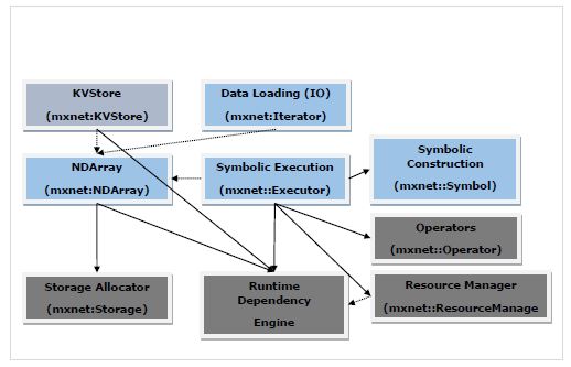
In the above diagram −
The modules in blue color boxes are User Facing Modules.
The modules in green color boxes are System Modules.
Solid arrow represents high dependency, i.e. heavily rely on the interface.
Dotted arrow represents light dependency, i.e. Used data structure for convenience and interface consistency. In fact, it can be replaced by the alternatives.
Let us discuss more about user facing and system modules.
User-facing Modules
The user-facing modules are as follows −
NDArray − It provides flexible imperative programs for Apache MXNet. They are dynamic and asynchronous n-dimensional arrays.
KVStore − It acts as interface for efficient parameter synchronization. In KVStore, KV stands for Key-Value. So, it a key-value store interface.
Data Loading (IO) − This user facing module is used for efficient distributed data loading and augmentation.
Symbol Execution − It is a static symbolic graph executor. It provides efficient symbolic graph execution and optimization.
Symbol Construction − This user facing module provides user a way to construct a computation graph i.e. net configuration.
System Modules
The system modules are as follows −
Storage Allocator − This system module, as name suggests, allocates and recycle memory blocks efficiently on host i.e. CPU and different devices i.e. GPUs.
Runtime Dependency Engine − Runtime dependency engine module schedules as well as executes the operations as per their read/write dependency.
Resource Manager − Resource Manager (RM) system module manages global resources like the random number generator and temporal space.
Operator − Operator system module consists of all the operators that define static forward and gradient calculation i.e. backpropagation.
Apache MXNet - System Components
Here, the system components in Apache MXNet are explained in detail. First, we will study about the execution engine in MXNet.
Execution Engine
Apache MXNets execution engine is very versatile. We can use it for deep learning as well as any domain-specific problem: execute a bunch of functions following their dependencies. It is designed in such a way that the functions with dependencies are serialized whereas, the functions with no dependencies can be executed in parallel.
Core Interface
The API given below is the core interface for Apache MXNets execution engine −
virtual void PushSync(Fn exec_fun, Context exec_ctx,
std::vector<VarHandle> const& const_vars,
std::vector<VarHandle> const& mutate_vars) = 0;
The above API has the following −
exec_fun − The core interface API of MXNet allows us to push the function named exec_fun, along with its context information and dependencies, to the execution engine.
exec_ctx − The context information in which the above-mentioned function exec_fun should be executed.
const_vars − These are the variables that the function reads from.
mutate_vars − These are the variables that are to be modified.
The execution engine provides its user the guarantee that the execution of any two functions that modify a common variable is serialized in their push order.
Function
Following is the function type of the execution engine of Apache MXNet −
using Fn = std::function<void(RunContext)>;
In the above function, RunContext contains the runtime information. The runtime information should be determined by the execution engine. The syntax of RunContext is as follows−
struct RunContext {
   // stream pointer which could be safely cast to
   // cudaStream_t* type
   void *stream;
};
Below are given some important points about execution engines functions −
All the functions are executed by MXNets execution engines internal threads.
It is not good to push blocking the function to the execution engine because with that the function will occupy the execution thread and will also reduce the total throughput.
For this MXNet provides another asynchronous function as follows−
using Callback = std::function<void()>;
using AsyncFn = std::function<void(RunContext, Callback)>;
In this AsyncFn function we can pass the heavy part of our threads, but the execution engine does not consider the function finished until we call the callback function.
Context
In Context, we can specify the context of the function to be executed within. This usually includes the following −
Whether the function should be run on a CPU or a GPU.
If we specify GPU in the Context, then which GPU to use.
There is a huge difference between Context and RunContext. Context have the device type and device id, whereas RunContext have the information that can be decided only during runtime.
VarHandle
VarHandle, used to specify the dependencies of functions, is like a token (especially provided by execution engine) we can use to represents the external resources the function can modify or use.
But the question arises, why we need to use VarHandle? It is because, the Apache MXNet engine is designed to decoupled from other MXNet modules.
Following are some important points about VarHandle −
It is lightweight so to create, delete, or copying a variable incurs little operating cost.
We need to specify the immutable variables i.e. the variables that will be used in the const_vars.
We need to specify the mutable variables i.e. the variables that will be modified in the mutate_vars.
The rule used by the execution engine to resolve the dependencies among functions is that the execution of any two functions when one of them modifies at least one common variable is serialized in their push order.
For creating a new variable, we can use the NewVar() API.
For deleting a variable, we can use the PushDelete API.
Let us understand its working with a simple example −
Suppose if we have two functions namely F1 and F2 and they both mutate the variable namely V2. In that case, F2 is guaranteed to be executed after F1 if F2 is pushed after F1. On the other side, if F1 and F2 both use V2 then their actual execution order could be random.
Push and Wait
Push and wait are two more useful API of execution engine.
Following are two important features of Push API:
All the Push APIs are asynchronous which means that the API call immediately returns regardless of whether the pushed function is finished or not.
Push API is not thread safe which means that only one thread should make engine API calls at a time.
Now if we talk about Wait API, following points represent it −
If a user wants to wait for a specific function to be finished, he/she should include a callback function in the closure. Once included, call the function at the end of the function.
On the other hand, if a user wants to wait for all functions that involves a certain variable to finish, he/she should use WaitForVar(var) API.
If someone wants to wait for all the pushed functions to finish, then use the WaitForAll () API.
Used to specify the dependencies of functions, is like a token.
Operators
Operator in Apache MXNet is a class that contains actual computation logic as well as auxiliary information and aid the system in performing optimisation.
Operator Interface
Forward is the core operator interface whose syntax is as follows:
virtual void Forward(const OpContext &ctx,
const std::vector<TBlob> &in_data,
const std::vector<OpReqType> &req,
const std::vector<TBlob> &out_data,
const std::vector<TBlob> &aux_states) = 0;
The structure of OpContext, defined in Forward() is as follows:
struct OpContext {
   int is_train;
   RunContext run_ctx;
   std::vector<Resource> requested;
}
The OpContext describes the state of operator (whether in the train or test phase), which device the operator should be run on and also the requested resources. two more useful API of execution engine.
From the above Forward core interface, we can understand the requested resources as follows −
in_data and out_data represent the input and output tensors.
req denotes how the result of computation are written into the out_data.
The OpReqType can be defined as −
enum OpReqType {
   kNullOp,
   kWriteTo,
   kWriteInplace,
   kAddTo
};
As like Forward operator, we can optionally implement the Backward interface as follows −
virtual void Backward(const OpContext &ctx,
const std::vector<TBlob> &out_grad,
const std::vector<TBlob> &in_data,
const std::vector<TBlob> &out_data,
const std::vector<OpReqType> &req,
const std::vector<TBlob> &in_grad,
const std::vector<TBlob> &aux_states);
Various tasks
Operator interface allows the users to do the following tasks −
User can specify in-place updates and can reduce memory allocation cost
In order to make it cleaner, the user can hide some internal arguments from Python.
User can define the relationship among the tensors and output tensors.
To perform computation, the user can acquire additional temporary space from the system.
Operator Property
As we are aware that in Convolutional neural network (CNN), one convolution has several implementations. To achieve the best performance from them, we might want to switch among those several convolutions.
That is the reason, Apache MXNet separate the operator semantic interface from the implementation interface. This separation is done in the form of OperatorProperty class which consists of the following−
InferShape − The InferShape interface has two purposes as given below:
First purpose is to tell the system the size of each input and output tensor so that the space can be allocated before Forward and Backward call.
Second purpose is to perform a size check to make sure that there is no error before running.
The syntax is given below −
virtual bool InferShape(mxnet::ShapeVector *in_shape,
mxnet::ShapeVector *out_shape,
mxnet::ShapeVector *aux_shape) const = 0;
Request Resource − What if your system can manage the computation workspace for operations like cudnnConvolutionForward? Your system can perform optimizations such as reuse the space and many more. Here, MXNet easily achieve this with the help of following two interfaces−
virtual std::vector<ResourceRequest> ForwardResource(
   const mxnet::ShapeVector &in_shape) const;
virtual std::vector<ResourceRequest> BackwardResource(
   const mxnet::ShapeVector &in_shape) const;
But, what if the ForwardResource and BackwardResource return non-empty arrays? In that case, the system offers corresponding resources through ctx parameter in the Forward and Backward interface of Operator.
Backward dependency − Apache MXNet has following two different operator signatures to deal with backward dependency −
void FullyConnectedForward(TBlob weight, TBlob in_data, TBlob out_data);
void FullyConnectedBackward(TBlob weight, TBlob in_data, TBlob out_grad, TBlob in_grad);
void PoolingForward(TBlob in_data, TBlob out_data);
void PoolingBackward(TBlob in_data, TBlob out_data, TBlob out_grad, TBlob in_grad);
Here, the two important points to note −
The out_data in FullyConnectedForward is not used by FullyConnectedBackward, and
PoolingBackward requires all the arguments of PoolingForward.
That is why for FullyConnectedForward, the out_data tensor once consumed could be safely freed because the backward function will not need it. With the help of this system got a to collect some tensors as garbage as early as possible.
In place Option − Apache MXNet provides another interface to the users to save the cost of memory allocation. The interface is appropriate for element-wise operations in which both input and output tensors have the same shape.
Following is the syntax for specifying the in-place update −
Example for Creating an Operator
With the help of OperatorProperty we can create an operator. To do so, follow the steps given below −
virtual std::vector<std::pair<int, void*>> ElewiseOpProperty::ForwardInplaceOption(
   const std::vector<int> &in_data,
   const std::vector<void*> &out_data)
const {
   return { {in_data[0], out_data[0]} };
}
virtual std::vector<std::pair<int, void*>> ElewiseOpProperty::BackwardInplaceOption(
   const std::vector<int> &out_grad,
   const std::vector<int> &in_data,
   const std::vector<int> &out_data,
   const std::vector<void*> &in_grad)
const {
   return { {out_grad[0], in_grad[0]} }
}
Step 1
Create Operator
First implement the following interface in OperatorProperty:
virtual Operator* CreateOperator(Context ctx) const = 0;
The example is given below −
class ConvolutionOp {
   public:
      void Forward( ... ) { ... }
      void Backward( ... ) { ... }
};
class ConvolutionOpProperty : public OperatorProperty {
   public:
      Operator* CreateOperator(Context ctx) const {
         return new ConvolutionOp;
      }
};
Step 2
Parameterize Operator
If you are going to implement a convolution operator, it is mandatory to know the kernel size, the stride size, padding size, and so on. Why, because these parameters should be passed to the operator before calling any Forward or backward interface.
For this, we need to define a ConvolutionParam structure as below −
#include <dmlc/parameter.h>
struct ConvolutionParam : public dmlc::Parameter<ConvolutionParam> {
   mxnet::TShape kernel, stride, pad;
   uint32_t num_filter, num_group, workspace;
   bool no_bias;
};
Now, we need to put this in ConvolutionOpProperty and pass it to the operator as follows −
class ConvolutionOp {
   public:
      ConvolutionOp(ConvolutionParam p): param_(p) {}
      void Forward( ... ) { ... }
      void Backward( ... ) { ... }
   private:
      ConvolutionParam param_;
};
class ConvolutionOpProperty : public OperatorProperty {
   public:
      void Init(const vector<pair<string, string>& kwargs) {
         // initialize param_ using kwargs
      }
      Operator* CreateOperator(Context ctx) const {
         return new ConvolutionOp(param_);
      }
   private:
      ConvolutionParam param_;
};
Step 3
Register the Operator Property Class and the Parameter Class to Apache MXNet
At last, we need to register the Operator Property Class and the Parameter Class to MXNet. It can be done with the help of following macros −
DMLC_REGISTER_PARAMETER(ConvolutionParam);
MXNET_REGISTER_OP_PROPERTY(Convolution, ConvolutionOpProperty);
In the above macro, the first argument is the name string and the second is the property class name.
Apache MXNet - Unified Operator API
This chapter provides information about the unified operator application programming interface (API) in Apache MXNet.
SimpleOp
SimpleOp is a new unified operator API which unifies different invoking processes. Once invoked, it returns to the fundamental elements of operators. The unified operator is specially designed for unary as well as binary operations. It is because most of the mathematical operators attend to one or two operands and more operands make the optimization, related to dependency, useful.
We will be understanding its SimpleOp unified operator working with the help of an example. In this example, we will be creating an operator functioning as a smooth l1 loss, which is a mixture of l1 and l2 loss. We can define and write the loss as given below −
loss = outside_weight .* f(inside_weight .* (data - label))
grad = outside_weight .* inside_weight .* f'(inside_weight .* (data - label))
Here, in above example,
.* stands for element-wise multiplication
f, f is the smooth l1 loss function which we are assuming is in mshadow.
It looks impossible to implement this particular loss as a unary or binary operator but MXNet provides its users automatic differentiation in symbolic execution which simplifies the loss to f and f directly. Thats why we can certainly implement this particular loss as a unary operator.
Defining Shapes
As we know MXNets mshadow library requires explicit memory allocation hence we need to provide all data shapes before any calculation occurs. Before defining functions and gradient, we need to provide input shape consistency and output shape as follows:
typedef mxnet::TShape (*UnaryShapeFunction)(const mxnet::TShape& src,
const EnvArguments& env);
   typedef mxnet::TShape (*BinaryShapeFunction)(const mxnet::TShape& lhs,
const mxnet::TShape& rhs,
const EnvArguments& env);
The function mxnet::Tshape is used to check input data shape and designated output data shape. In case, if you do not define this function then the default output shape would be same as input shape. For example, in case of binary operator the shape of lhs and rhs is by default checked as the same.
Now lets move on to our smooth l1 loss example. For this, we need to define an XPU to cpu or gpu in the header implementation smooth_l1_unary-inl.h. The reason is to reuse the same code in smooth_l1_unary.cc and smooth_l1_unary.cu.
#include <mxnet/operator_util.h>
   #if defined(__CUDACC__)
      #define XPU gpu
   #else
      #define XPU cpu
#endif
As in our smooth l1 loss example, the output has the same shape as the source, we can use the default behavior. It can be written as follows −
inline mxnet::TShape SmoothL1Shape_(const mxnet::TShape& src,const EnvArguments& env) {
   return mxnet::TShape(src);
}
Defining Functions
We can create a unary or binary function with one input as follows −
typedef void (*UnaryFunction)(const TBlob& src,
   const EnvArguments& env,
   TBlob* ret,
   OpReqType req,
   RunContext ctx);
typedef void (*BinaryFunction)(const TBlob& lhs,
   const TBlob& rhs,
   const EnvArguments& env,
   TBlob* ret,
   OpReqType req,
   RunContext ctx);
Following is the RunContext ctx struct which contains the information needed during runtime for execution −
struct RunContext {
   void *stream; // the stream of the device, can be NULL or Stream<gpu>* in GPU mode
   template<typename xpu> inline mshadow::Stream<xpu>* get_stream() // get mshadow stream from Context
} // namespace mxnet
Now, lets see how we can write the computation results in ret.
enum OpReqType {
   kNullOp, // no operation, do not write anything
   kWriteTo, // write gradient to provided space
   kWriteInplace, // perform an in-place write
   kAddTo // add to the provided space
};
Now, lets move on to our smooth l1 loss example. For this, we will use UnaryFunction to define the function of this operator as follows:
template<typename xpu>
void SmoothL1Forward_(const TBlob& src,
   const EnvArguments& env,
   TBlob *ret,
   OpReqType req,
RunContext ctx) {
   using namespace mshadow;
   using namespace mshadow::expr;
   mshadow::Stream<xpu> *s = ctx.get_stream<xpu>();
   real_t sigma2 = env.scalar * env.scalar;
   MSHADOW_TYPE_SWITCH(ret->type_flag_, DType, {
      mshadow::Tensor<xpu, 2, DType> out = ret->get<xpu, 2, DType>(s);
      mshadow::Tensor<xpu, 2, DType> in = src.get<xpu, 2, DType>(s);
      ASSIGN_DISPATCH(out, req,
      F<mshadow_op::smooth_l1_loss>(in, ScalarExp<DType>(sigma2)));
   });
}
Defining Gradients
Except Input, TBlob, and OpReqType are doubled, Gradients functions of binary operators have similar structure. Lets check out below, where we created a gradient function with various types of input:
// depending only on out_grad
typedef void (*UnaryGradFunctionT0)(const OutputGrad& out_grad,
   const EnvArguments& env,
   TBlob* in_grad,
   OpReqType req,
   RunContext ctx);
// depending only on out_value
typedef void (*UnaryGradFunctionT1)(const OutputGrad& out_grad,
   const OutputValue& out_value,
   const EnvArguments& env,
   TBlob* in_grad,
   OpReqType req,
   RunContext ctx);
// depending only on in_data
typedef void (*UnaryGradFunctionT2)(const OutputGrad& out_grad,
   const Input0& in_data0,
   const EnvArguments& env,
   TBlob* in_grad,
   OpReqType req,
   RunContext ctx);
As defined above Input0, Input, OutputValue, and OutputGrad all share the structure of GradientFunctionArgument. It is defined as follows −
struct GradFunctionArgument {
   TBlob data;
}
Now lets move on to our smooth l1 loss example. For this to enable the chain rule of gradient we need to multiply out_grad from the top to the result of in_grad.
template<typename xpu>
void SmoothL1BackwardUseIn_(const OutputGrad& out_grad, const Input0& in_data0,
   const EnvArguments& env,
   TBlob *in_grad,
   OpReqType req,
   RunContext ctx) {
   using namespace mshadow;
   using namespace mshadow::expr;
   mshadow::Stream<xpu> *s = ctx.get_stream<xpu>();
   real_t sigma2 = env.scalar * env.scalar;
      MSHADOW_TYPE_SWITCH(in_grad->type_flag_, DType, {
      mshadow::Tensor<xpu, 2, DType> src = in_data0.data.get<xpu, 2, DType>(s);
      mshadow::Tensor<xpu, 2, DType> ograd = out_grad.data.get<xpu, 2, DType>(s);
      mshadow::Tensor<xpu, 2, DType> igrad = in_grad->get<xpu, 2, DType>(s);
      ASSIGN_DISPATCH(igrad, req,
      ograd * F<mshadow_op::smooth_l1_gradient>(src, ScalarExp<DType>(sigma2)));
   });
}
Register SimpleOp to MXNet
Once we created the shape, function, and gradient, we need to restore them into both an NDArray operator as well as into a symbolic operator. For this, we can use the registration macro as follows −
MXNET_REGISTER_SIMPLE_OP(Name, DEV)
   .set_shape_function(Shape)
   .set_function(DEV::kDevMask, Function<XPU>, SimpleOpInplaceOption)
   .set_gradient(DEV::kDevMask, Gradient<XPU>, SimpleOpInplaceOption)
   .describe("description");
The SimpleOpInplaceOption can be defined as follows −
enum SimpleOpInplaceOption {
   kNoInplace, // do not allow inplace in arguments
   kInplaceInOut, // allow inplace in with out (unary)
   kInplaceOutIn, // allow inplace out_grad with in_grad (unary)
   kInplaceLhsOut, // allow inplace left operand with out (binary)

   kInplaceOutLhs // allow inplace out_grad with lhs_grad (binary)
};
Now lets move on to our smooth l1 loss example. For this, we have a gradient function that relies on input data so that the function cannot be written in place.
MXNET_REGISTER_SIMPLE_OP(smooth_l1, XPU)
.set_function(XPU::kDevMask, SmoothL1Forward_<XPU>, kNoInplace)
.set_gradient(XPU::kDevMask, SmoothL1BackwardUseIn_<XPU>, kInplaceOutIn)
.set_enable_scalar(true)
.describe("Calculate Smooth L1 Loss(lhs, scalar)");
SimpleOp on EnvArguments
As we know some operations might need the following −
A scalar as input such as a gradient scale
A set of keyword arguments controlling behavior
A temporary space to speed up calculations.
The benefit of using EnvArguments is that it provides additional arguments and resources to make calculations more scalable and efficient.
Example
First lets define the struct as below −
struct EnvArguments {
   real_t scalar; // scalar argument, if enabled
   std::vector<std::pair<std::string, std::string> > kwargs; // keyword arguments
   std::vector<Resource> resource; // pointer to the resources requested
};
Next, we need to request additional resources like mshadow::Random<xpu> and temporary memory space from EnvArguments.resource. It can be done as follows −
struct ResourceRequest {
   enum Type { // Resource type, indicating what the pointer type is
      kRandom, // mshadow::Random<xpu> object
      kTempSpace // A dynamic temp space that can be arbitrary size
   };
   Type type; // type of resources
};
Now, the registration will request the declared resource request from mxnet::ResourceManager. After that, it will place the resources in std::vector<Resource> resource in EnvAgruments.
We can access the resources with the help of following code −
auto tmp_space_res = env.resources[0].get_space(some_shape, some_stream);
auto rand_res = env.resources[0].get_random(some_stream);
If you see in our smooth l1 loss example, a scalar input is needed to mark the turning point of a loss function. Thats why in the registration process, we use set_enable_scalar(true), and env.scalar in function and gradient declarations.
Building Tensor Operation
Here the question arises that why we need to craft tensor operations? The reasons are as follows −
Computation utilizes the mshadow library and we sometimes do not have functions readily available.
If an operation is not done in an element-wise way such as softmax loss and gradient.
Example
Here, we are using the above smooth l1 loss example. We will be creating two mappers namely the scalar cases of smooth l1 loss and gradient:
namespace mshadow_op {
   struct smooth_l1_loss {
      // a is x, b is sigma2
      MSHADOW_XINLINE static real_t Map(real_t a, real_t b) {
         if (a > 1.0f / b) {
            return a - 0.5f / b;
         } else if (a < -1.0f / b) {
            return -a - 0.5f / b;
         } else {
            return 0.5f * a * a * b;
         }
      }
   };
}
Apache MXNet - Distributed Training
This chapter is about the distributed training in Apache MXNet. Let us start by understanding what are the modes of computation in MXNet.
Modes of Computation
MXNet, a multi-language ML library, offers its users the following two modes of computation −
Imperative mode
This mode of computation exposes an interface like NumPy API. For example, in MXNet, use the following imperative code to construct a tensor of zeros on both CPU as well as GPU −
import mxnet as mx
tensor_cpu = mx.nd.zeros((100,), ctx=mx.cpu())
tensor_gpu= mx.nd.zeros((100,), ctx=mx.gpu(0))
As we see in the above code, MXNets specifies the location where to hold the tensor, either in CPU or GPU device. In above example, it is at location 0. MXNet achieve incredible utilisation of the device, because all the computations happen lazily instead of instantaneously.
Symbolic mode
Although the imperative mode is quite useful, but one of the drawbacks of this mode is its rigidity, i.e. all the computations need to be known beforehand along with pre-defined data structures.
On the other hand, Symbolic mode exposes a computation graph like TensorFlow. It removes the drawback of imperative API by allowing MXNet to work with symbols or variables instead of fixed/pre-defined data structures. Afterwards, the symbols can be interpreted as a set of operations as follows −
import mxnet as mx
x = mx.sym.Variable(X)
y = mx.sym.Variable(Y)
z = (x+y)
m = z/100
Kinds of Parallelism
Apache MXNet supports distributed training. It enables us to leverage multiple machines for faster as well as effective training.
Following are the two ways in which, we can distribute the workload of training a NN across multiple devices, CPU or GPU device −
Data Parallelism
In this kind of parallelism, each device stores a complete copy of the model and works with a different part of the dataset. Devices also update a shared model collectively. We can locate all the devices on a single machine or across multiple machines.
Model Parallelism
It is another kind of parallelism, which comes handy when models are so large that they do not fit into device memory. In model parallelism, different devices are assigned the task of learning different parts of the model. The important point here to note is that currently Apache MXNet supports model parallelism in a single machine only.
Working of distributed training
The concepts given below are the key to understand the working of distributed training in Apache MXNet −
Types of processes
Processes communicates with each other to accomplish the training of a model. Apache MXNet has the following three processes −
Worker
The job of worker node is to perform training on a batch of training samples. The Worker nodes will pull weights from the server before processing every batch. The Worker nodes will send gradients to the server, once the batch is processed.
Server
MXNet can have multiple servers for storing the models parameters and to communicate with the worker nodes.
Scheduler
The role of the scheduler is to set up the cluster, which includes waiting for messages that each node has come up and which port the node is listening to. After setting up the cluster, the scheduler lets all the processes know about every other node in the cluster. It is because the processes can communicate with each other. There is only one scheduler.
KV Store
KV stores stands for Key-Value store. It is critical component used for multi-device training. It is important because, the communication of parameters across devices on single as well as across multiple machines is transmitted through one or more servers with a KVStore for the parameters. Lets understand the working of KVStore with the help of following points −
Each value in KVStore is represented by a key and a value.
Each parameter array in the network is assigned a key and the weights of that parameter array is referred by value.
After that, the worker nodes push gradients after processing a batch. They also pull updated weights before processing a new batch.
The notion of KVStore server exists only during distributed training and the distributed mode of it is enabled by calling mxnet.kvstore.create function with a string argument containing the word dist −
kv = mxnet.kvstore.create(dist_sync)
Distribution of Keys
It is not necessary that, all the servers store all the parameters array or keys, but they are distributed across different servers. Such distribution of keys across different servers is handled transparently by the KVStore and the decision of which server stores a specific key is made at random.
KVStore, as discussed above, ensures that whenever the key is pulled, its request is sent to that server, which has the corresponding value. What if the value of some key is large? In that case, it may be shared across different servers.
Split training data
As being the users, we want each machine to be working on different parts of the dataset, especially, when running distributed training in data parallel mode. We know that, to split a batch of samples provided by the data iterator for data parallel training on a single worker we can use mxnet.gluon.utils.split_and_load and then, load each part of the batch on the device which will process it further.
On the other hand, in case of distributed training, at beginning we need to divide the dataset into n different parts so that every worker gets a different part. Once got, each worker can then use split_and_load to again divide that part of the dataset across different devices on a single machine. All this happen through data iterator. mxnet.io.MNISTIterator and mxnet.io.ImageRecordIter are two such iterators in MXNet that support this feature.
Weights updating
For updating the weights, KVStore supports following two modes −
First method aggregates the gradients and updates the weights by using those gradients.
In the second method the server only aggregates gradients.
If you are using Gluon, there is an option to choose between above stated methods by passing update_on_kvstore variable. Lets understand it by creating the trainer object as follows −
trainer = gluon.Trainer(net.collect_params(), optimizer='sgd',
   optimizer_params={'learning_rate': opt.lr,
      'wd': opt.wd,
      'momentum': opt.momentum,
      'multi_precision': True},
      kvstore=kv,
   update_on_kvstore=True)
Modes of Distributed Training
If the KVStore creation string contains the word dist, it means the distributed training is enabled. Following are different modes of distributed training that can be enabled by using different types of KVStore −
dist_sync
As name implies, it denotes synchronous distributed training. In this, all the workers use the same synchronized set of model parameters at the start of every batch.
The drawback of this mode is that, after each batch the server should have to wait to receive gradients from each worker before it updates the model parameters. This means that if a worker crashes, it would halt the progress of all workers.
dist_async
As name implies, it denotes synchronous distributed training. In this, the server receives gradients from one worker and immediately updates its store. Server uses the updated store to respond to any further pulls.
The advantage, in comparison of dist_sync mode, is that a worker who finishes processing a batch can pull the current parameters from server and start the next batch. The worker can do so, even if the other worker has not yet finished processing the earlier batch. It is also faster than dist_sync mode because, it can take more epochs to converge without any cost of synchronization.
dist_sync_device
This mode is same as dist_sync mode. The only difference is that, when there are multiple GPUs being used on every node dist_sync_device aggregates gradients and updates weights on GPU whereas, dist_sync aggregates gradients and updates weights on CPU memory.
It reduces expensive communication between GPU and CPU. That is why, it is faster than dist_sync. The drawback is that it increases the memory usage on GPU.
dist_async_device
This mode works same as dist_sync_device mode, but in asynchronous mode.
Apache MXNet - Python Packages
In this chapter we will learn about the Python Packages available in Apache MXNet.
Important MXNet Python packages
MXNet has the following important Python packages which we will be discussing one by one −
Autograd (Automatic Differentiation)
NDArray
KVStore
Gluon
Visualization
First let us start with Autograd Python package for Apache MXNet.
Autograd
Autograd stands for automatic differentiation used to backpropagate the gradients from the loss metric back to each of the parameters. Along with backpropagation it uses a dynamic programming approach to efficiently calculate the gradients. It is also called reverse mode automatic differentiation. This technique is very efficient in fan-in situations where, many parameters effect a single loss metric.
What are gradients?
Gradients are the fundamentals to the process of neural network training. They basically tell us how to change the parameters of the network to improve its performance.
As we know that, neural networks (NN) are composed of operators such as sums, product, convolutions, etc. These operators, for their computations, use parameters such as the weights in convolution kernels. We should have to find the optimal values for these parameters and gradients shows us the way and lead us to the solution as well.
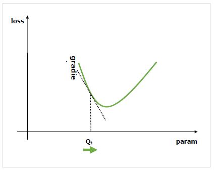
We are interested in the effect of changing a parameter on performance of the network and gradients tell us, how much a given variable increases or decreases when we change a variable it depends on. The performance is usually defined by using a loss metric that we try to minimise. For example, for regression we might try to minimise L2 loss between our predictions and exact value, whereas for classification we might minimise the cross-entropy loss.
Once we calculate the gradient of each parameter with reference to the loss, we can then use an optimiser, such as stochastic gradient descent.
How to calculate gradients?
We have the following options to calculate gradients −
Symbolic Differentiation − The very first option is Symbolic Differentiation, which calculates the formulas for each gradient. The drawback of this method is that, it will quickly lead to incredibly long formulas as the network get deeper and operators get more complex.
Finite Differencing − Another option is, to use finite differencing which try slight differences on each parameter and see how the loss metric responds. The drawback of this method is that, it would be computationally expensive and may have poor numerical precision.
Automatic differentiation − The solution to the drawbacks of the above methods is, to use automatic differentiation to backpropagate the gradients from the loss metric back to each of the parameters. Propagation allows us a dynamic programming approach to efficiently calculate the gradients. This method is also called reverse mode automatic differentiation.
Automatic Differentiation (autograd)
Here, we will understand in detail the working of autograd. It basically works in following two stages −
Stage 1 − This stage is called Forward Pass of training. As name implies, in this stage it creates the record of the operator used by the network to make predictions and calculate the loss metric.
Stage 2 − This stage is called Backward Pass of training. As name implies, in this stage it works backwards through this record. Going backwards, it evaluates the partial derivatives of each operator, all the way back to the network parameter.
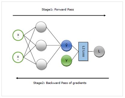
Advantages of autograd
Following are the advantages of using Automatic Differentiation (autograd) −
Flexible − Flexibility, that it gives us when defining our network, is one of the huge benefits of using autograd. We can change the operations on every iteration. These are called the dynamic graphs, which are much more complex to implement in frameworks requiring static graph. Autograd, even in such cases, will still be able to backpropagate the gradients correctly.
Automatic − Autograd is automatic, i.e. the complexities of the backpropagation procedure are taken care of by it for you. We just need to specify what gradients we are interested in calculating.
Efficient − Autogard calculates the gradients very efficiently.
Can use native Python control flow operators − We can use the native Python control flow operators such as if condition and while loop. The autograd will still be able to backpropagate the gradients efficiently and correctly.
Using autograd in MXNet Gluon
Here, with the help of an example, we will see how we can use autograd in MXNet Gluon.
Implementation Example
In the following example, we will implement the regression model having two layers. After implementing, we will use autograd to automatically calculate the gradient of the loss with reference to each of the weight parameters −
First import the autogrard and other required packages as follows −
from mxnet import autograd
import mxnet as mx
from mxnet.gluon.nn import HybridSequential, Dense
from mxnet.gluon.loss import L2Loss
Now, we need to define the network as follows −
N_net = HybridSequential()
N_net.add(Dense(units=3))
N_net.add(Dense(units=1))
N_net.initialize()
Now we need to define the loss as follows −
loss_function = L2Loss()
Next, we need to create the dummy data as follows −
x = mx.nd.array([[0.5, 0.9]])
y = mx.nd.array([[1.5]])
Now, we are ready for our first forward pass through the network. We want autograd to record the computational graph so that we can calculate the gradients. For this, we need to run the network code in the scope of autograd.record context as follows −
with autograd.record():
   y_hat = N_net(x)
   loss = loss_function(y_hat, y)
Now, we are ready for the backward pass, which we start by calling the backward method on the quantity of interest. The quatity of interest in our example is loss because we are trying to calculate the gradient of loss with reference to the parameters −
loss.backward()
Now, we have gradients for each parameter of the network, which will be used by the optimiser to update the parameter value for improved performance. Lets check out the gradients of the 1st layer as follows −
N_net[0].weight.grad()
Output
The output is as follows−
[[-0.00470527 -0.00846948]
[-0.03640365 -0.06552657]
[ 0.00800354 0.01440637]]
<NDArray 3x2 @cpu(0)>
Complete implementation example
Given below is the complete implementation example.
from mxnet import autograd
import mxnet as mx
from mxnet.gluon.nn import HybridSequential, Dense
from mxnet.gluon.loss import L2Loss
N_net = HybridSequential()
N_net.add(Dense(units=3))
N_net.add(Dense(units=1))
N_net.initialize()
loss_function = L2Loss()
x = mx.nd.array([[0.5, 0.9]])
y = mx.nd.array([[1.5]])
with autograd.record():
y_hat = N_net(x)
loss = loss_function(y_hat, y)
loss.backward()
N_net[0].weight.grad()
Apache MXNet - NDArray
In this chapter, we will be discussing about MXNets multi-dimensional array format called ndarray.
Handling data with NDArray
First, we are going see how we can handle data with NDArray. Following are the prerequisites for the same −
Prerequisites
To understand how we can handle data with this multi-dimensional array format, we need to fulfil the following prerequisites:
MXNet installed in a Python environment
Python 2.7.x or Python 3.x
Implementation Example
Let us understand the basic functionality with the help of an example given below −
First, we need to import MXNet and ndarray from MXNet as follows −
import mxnet as mx
from mxnet import nd
Once we import the necessary libraries, we will go with the following basic functionalities:
A simple 1-D array with a python list
Example
x = nd.array([1,2,3,4,5,6,7,8,9,10])
print(x)
Output
The output is as mentioned below −
[ 1. 2. 3. 4. 5. 6. 7. 8. 9. 10.]
<NDArray 10 @cpu(0)>
A 2-D array with a python list
Example
y = nd.array([[1,2,3,4,5,6,7,8,9,10], [1,2,3,4,5,6,7,8,9,10], [1,2,3,4,5,6,7,8,9,10]])
print(y)
Output
The output is as stated below −
[[ 1. 2. 3. 4. 5. 6. 7. 8. 9. 10.]
[ 1. 2. 3. 4. 5. 6. 7. 8. 9. 10.]
[ 1. 2. 3. 4. 5. 6. 7. 8. 9. 10.]]
<NDArray 3x10 @cpu(0)>
Creating an NDArray without any initialisation
Here, we will create a matrix with 3 rows and 4 columns by using .empty function. We will also use .full function, which will take an additional operator for what value you want to fill in the array.
Example
x = nd.empty((3, 4))
print(x)
x = nd.full((3,4), 8)
print(x)
Output
The output is given below −
[[0.000e+00 0.000e+00 0.000e+00 0.000e+00]
 [0.000e+00 0.000e+00 2.887e-42 0.000e+00]
 [0.000e+00 0.000e+00 0.000e+00 0.000e+00]]
<NDArray 3x4 @cpu(0)>

[[8. 8. 8. 8.]
 [8. 8. 8. 8.]
 [8. 8. 8. 8.]]
<NDArray 3x4 @cpu(0)>
Matrix of all zeros with the .zeros function
Example
x = nd.zeros((3, 8))
print(x)
Output
The output is as follows −
[[0. 0. 0. 0. 0. 0. 0. 0.]
 [0. 0. 0. 0. 0. 0. 0. 0.]
 [0. 0. 0. 0. 0. 0. 0. 0.]]
<NDArray 3x8 @cpu(0)>
Matrix of all ones with the .ones function
Example
x = nd.ones((3, 8))
print(x)
Output
The output is mentioned below −
[[1. 1. 1. 1. 1. 1. 1. 1.]
   [1. 1. 1. 1. 1. 1. 1. 1.]
   [1. 1. 1. 1. 1. 1. 1. 1.]]
<NDArray 3x8 @cpu(0)>
Creating array whose values are sampled randomly
Example
y = nd.random_normal(0, 1, shape=(3, 4))
print(y)
Output
The output is given below −
[[ 1.2673576 -2.0345826 -0.32537818 -1.4583491 ]
 [-0.11176403 1.3606371 -0.7889914 -0.17639421]
 [-0.2532185 -0.42614475 -0.12548696 1.4022992 ]]
<NDArray 3x4 @cpu(0)>
Finding dimension of each NDArray
Example
y.shape
Output
The output is as follows −
(3, 4)
Finding the size of each NDArray
Example
y.size
Output
12
Finding the datatype of each NDArray
Example
y.dtype
Output
numpy.float32
NDArray Operations
In this section, we will introduce you to MXNets array operations. NDArray support large number of standard mathematical as well as In-place operations.
Standard Mathematical Operations
Following are standard mathematical operations supported by NDArray −
Element-wise addition
First, we need to import MXNet and ndarray from MXNet as follows:
import mxnet as mx
from mxnet import nd
x = nd.ones((3, 5))
y = nd.random_normal(0, 1, shape=(3, 5))
print('x=', x)
print('y=', y)
x = x + y
print('x = x + y, x=', x)
Output
The output is given herewith −
x=
[[1. 1. 1. 1. 1.]
[1. 1. 1. 1. 1.]
[1. 1. 1. 1. 1.]]
<NDArray 3x5 @cpu(0)>
y=
[[-1.0554522 -1.3118273 -0.14674698 0.641493 -0.73820823]
[ 2.031364 0.5932667 0.10228804 1.179526 -0.5444829 ]
[-0.34249446 1.1086396 1.2756858 -1.8332436 -0.5289873 ]]
<NDArray 3x5 @cpu(0)>
x = x + y, x=
[[-0.05545223 -0.3118273 0.853253 1.6414931 0.26179177]
[ 3.031364 1.5932667 1.102288 2.1795259 0.4555171 ]
[ 0.6575055 2.1086397 2.2756858 -0.8332436 0.4710127 ]]
<NDArray 3x5 @cpu(0)>
Element-wise multiplication
Example
x = nd.array([1, 2, 3, 4])
y = nd.array([2, 2, 2, 1])
x * y
Output
You will see the following output−
[2. 4. 6. 4.]
<NDArray 4 @cpu(0)>
Exponentiation
Example
nd.exp(x)
Output
When you run the code, you will see the following output:
[ 2.7182817 7.389056 20.085537 54.59815 ]
<NDArray 4 @cpu(0)>
Matrix transpose to compute matrix-matrix product
Example
nd.dot(x, y.T)
Output
Given below is the output of the code −
[16.]
<NDArray 1 @cpu(0)>
In-place Operations
Every time, in the above example, we ran an operation, we allocated a new memory to host its result.
For example, if we write A = A+B, we will dereference the matrix that A used to point to and instead point it at the newly allocated memory. Let us understand it with the example given below, using Pythons id() function −
print('y=', y)
print('id(y):', id(y))
y = y + x
print('after y=y+x, y=', y)
print('id(y):', id(y))
Output
Upon execution, you will receive the following output −
y=
[2. 2. 2. 1.]
<NDArray 4 @cpu(0)>
id(y): 2438905634376
after y=y+x, y=
[3. 4. 5. 5.]
<NDArray 4 @cpu(0)>
id(y): 2438905685664
In fact, we can also assign the result to a previously allocated array as follows −
print('x=', x)
z = nd.zeros_like(x)
print('z is zeros_like x, z=', z)
print('id(z):', id(z))
print('y=', y)
z[:] = x + y
print('z[:] = x + y, z=', z)
print('id(z) is the same as before:', id(z))
Output
The output is shown below −
x=
[1. 2. 3. 4.]
<NDArray 4 @cpu(0)>
z is zeros_like x, z=
[0. 0. 0. 0.]
<NDArray 4 @cpu(0)>
id(z): 2438905790760
y=
[3. 4. 5. 5.]
<NDArray 4 @cpu(0)>
z[:] = x + y, z=
[4. 6. 8. 9.]
<NDArray 4 @cpu(0)>
id(z) is the same as before: 2438905790760
From the above output, we can see that x+y will still allocate a temporary buffer to store the result before copying it to z. So now, we can perform operations in-place to make better use of memory and to avoid temporary buffer. To do this, we will specify the out keyword argument every operator support as follows −
print('x=', x, 'is in id(x):', id(x))
print('y=', y, 'is in id(y):', id(y))
print('z=', z, 'is in id(z):', id(z))
nd.elemwise_add(x, y, out=z)
print('after nd.elemwise_add(x, y, out=z), x=', x, 'is in id(x):', id(x))
print('after nd.elemwise_add(x, y, out=z), y=', y, 'is in id(y):', id(y))
print('after nd.elemwise_add(x, y, out=z), z=', z, 'is in id(z):', id(z))
Output
On executing the above program, you will get the following result −
x=
[1. 2. 3. 4.]
<NDArray 4 @cpu(0)> is in id(x): 2438905791152
y=
[3. 4. 5. 5.]
<NDArray 4 @cpu(0)> is in id(y): 2438905685664
z=
[4. 6. 8. 9.]
<NDArray 4 @cpu(0)> is in id(z): 2438905790760
after nd.elemwise_add(x, y, out=z), x=
[1. 2. 3. 4.]
<NDArray 4 @cpu(0)> is in id(x): 2438905791152
after nd.elemwise_add(x, y, out=z), y=
[3. 4. 5. 5.]
<NDArray 4 @cpu(0)> is in id(y): 2438905685664
after nd.elemwise_add(x, y, out=z), z=
[4. 6. 8. 9.]
<NDArray 4 @cpu(0)> is in id(z): 2438905790760
NDArray Contexts
In Apache MXNet, each array has a context and one context could be the CPU, whereas other contexts might be several GPUs. The things can get even worst, when we deploy the work across multiple servers. Thats why, we need to assign arrays to contexts intelligently. It will minimise the time spent transferring data between devices.
For example, try initialising an array as follows −
from mxnet import nd
z = nd.ones(shape=(3,3), ctx=mx.cpu(0))
print(z)
Output
When you execute the above code, you should see the following output −
[[1. 1. 1.]
 [1. 1. 1.]
 [1. 1. 1.]]
<NDArray 3x3 @cpu(0)>
We can copy the given NDArray from one context to another context by using the copyto() method as follows −
x_gpu = x.copyto(gpu(0))
print(x_gpu)
NumPy array vs. NDArray
We all the familiar with NumPy arrays but Apache MXNet offers its own array implementation named NDArray. Actually, it was initially designed to be similar to NumPy but there is a key difference −
The key difference is in the way calculations are executed in NumPy and NDArray. Every NDArray manipulation in MXNet is done in asynchronous and non-blocking way, which means that, when we write code like c = a * b, the function is pushed to the Execution Engine, which will start the calculation.
Here, a and b both are NDArrays. The benefit of using it is that, the function immediately returns back, and the user thread can continue execution despite the fact that the previous calculation may not have been completed yet.
Working of Execution Engine
If we talk about the working of execution engine, it builds the computation graph. The computation graph may reorder or combine some calculations, but it always honors dependency order.
For example, if there are other manipulation with X done later in the programming code, the Execution Engine will start doing them once the result of X is available. Execution engine will handle some important works for the users, such as writing of callbacks to start execution of subsequent code.
In Apache MXNet, with the help of NDArray, to get the result of computation we only need to access the resulting variable. The flow of the code will be blocked until the computation results are assigned to the resulting variable. In this way, it increases code performance while still supporting imperative programming mode.
Converting NDArray to NumPy Array
Let us learn how can we convert NDArray to NumPy Array in MXNet.
Combining higher-level operator with the help of few lower-level operators
Sometimes, we can assemble a higher-level operator by using the existing operators. One of the best examples of this is, the np.full_like() operator, which is not there in NDArray API. It can easily be replaced with a combination of existing operators as follows:
from mxnet import nd
import numpy as np
np_x = np.full_like(a=np.arange(7, dtype=int), fill_value=15)
nd_x = nd.ones(shape=(7,)) * 15
np.array_equal(np_x, nd_x.asnumpy())
Output
We will get the output similar as follows −
True
Finding similar operator with different name and/or signature
Among all the operators, some of them have slightly different name, but they are similar in the terms of functionality. An example of this is nd.ravel_index() with np.ravel() functions. In the same way, some operators may have similar names, but they have different signatures. An example of this is np.split() and nd.split() are similar.
Lets understand it with the following programming example:
def pad_array123(data, max_length):
data_expanded = data.reshape(1, 1, 1, data.shape[0])
data_padded = nd.pad(data_expanded,
mode='constant',
pad_width=[0, 0, 0, 0, 0, 0, 0, max_length - data.shape[0]],
constant_value=0)
data_reshaped_back = data_padded.reshape(max_length)
return data_reshaped_back
pad_array123(nd.array([1, 2, 3]), max_length=10)
Output
The output is stated below −
[1. 2. 3. 0. 0. 0. 0. 0. 0. 0.]
<NDArray 10 @cpu(0)>
Minimising impact of blocking calls
In some of the cases, we have to use either .asnumpy() or .asscalar() methods, but this will force MXNet to block the execution, until the result can be retrieved. We can minimise the impact of a blocking call by calling .asnumpy() or .asscalar() methods in the moment, when we think the calculation of this value is already done.
Implementation Example
Example
from __future__ import print_function
import mxnet as mx
from mxnet import gluon, nd, autograd
from mxnet.ndarray import NDArray
from mxnet.gluon import HybridBlock
import numpy as np

class LossBuffer(object):
   """
   Simple buffer for storing loss value
   """

   def __init__(self):
      self._loss = None

   def new_loss(self, loss):
      ret = self._loss
      self._loss = loss
      return ret

      @property
      def loss(self):
         return self._loss

net = gluon.nn.Dense(10)
ce = gluon.loss.SoftmaxCELoss()
net.initialize()
data = nd.random.uniform(shape=(1024, 100))
label = nd.array(np.random.randint(0, 10, (1024,)), dtype='int32')
train_dataset = gluon.data.ArrayDataset(data, label)
train_data = gluon.data.DataLoader(train_dataset, batch_size=128, shuffle=True, num_workers=2)
trainer = gluon.Trainer(net.collect_params(), optimizer='sgd')
loss_buffer = LossBuffer()
for data, label in train_data:
   with autograd.record():
      out = net(data)
      # This call saves new loss and returns previous loss
      prev_loss = loss_buffer.new_loss(ce(out, label))
   loss_buffer.loss.backward()
   trainer.step(data.shape[0])
   if prev_loss is not None:
      print("Loss: {}".format(np.mean(prev_loss.asnumpy())))
Output
The output is cited below:
Loss: 2.3373236656188965
Loss: 2.3656985759735107
Loss: 2.3613128662109375
Loss: 2.3197104930877686
Loss: 2.3054862022399902
Loss: 2.329197406768799
Loss: 2.318927526473999
Apache MXNet - Gluon
Another most important MXNet Python package is Gluon. In this chapter, we will be discussing this package. Gluon provides a clear, concise, and simple API for DL projects. It enables Apache MXNet to prototype, build, and train DL models without forfeiting the training speed.
Blocks
Blocks form the basis of more complex network designs. In a neural network, as the complexity of neural network increases, we need to move from designing single to entire layers of neurons. For example, NN design like ResNet-152 have a very fair degree of regularity by consisting of blocks of repeated layers.
Example
In the example given below, we will write code a simple block, namely block for a multilayer perceptron.
from mxnet import nd
from mxnet.gluon import nn
x = nd.random.uniform(shape=(2, 20))
N_net = nn.Sequential()
N_net.add(nn.Dense(256, activation='relu'))
N_net.add(nn.Dense(10))
N_net.initialize()
N_net(x)
Output
This produces the following output:
[[ 0.09543004 0.04614332 -0.00286655 -0.07790346 -0.05130241 0.02942038
0.08696645 -0.0190793 -0.04122177 0.05088576]
[ 0.0769287 0.03099706 0.00856576 -0.044672 -0.06926838 0.09132431
0.06786592 -0.06187843 -0.03436674 0.04234696]]
<NDArray 2x10 @cpu(0)>
Steps needed to go from defining layers to defining blocks of one or more layers −
Step 1 − Block take the data as input.
Step 2 − Now, blocks will store the state in the form of parameters. For example, in the above coding example the block contains two hidden layers and we need a place to store parameters for it.
Step 3 − Next block will invoke the forward function to perform forward propagation. It is also called forward computation. As a part of first forward call, blocks initialize the parameters in a lazy fashion.
Step 4 − At last the blocks will invoke backward function and calculate the gradient with reference to their input. Typically, this step is performed automatically.
Sequential Block
A sequential block is a special kind of block in which the data flows through a sequence of blocks. In this, each block applied to the output of one before with the first block being applied on the input data itself.
Let us see how sequential class works −
from mxnet import nd
from mxnet.gluon import nn
class MySequential(nn.Block):
   def __init__(self, **kwargs):
      super(MySequential, self).__init__(**kwargs)

   def add(self, block):
      self._children[block.name] = block
   def forward(self, x):
   for block in self._children.values():
      x = block(x)
   return x
x = nd.random.uniform(shape=(2, 20))
N_net = MySequential()
N_net.add(nn.Dense(256, activation
='relu'))
N_net.add(nn.Dense(10))
N_net.initialize()
N_net(x)
Output
The output is given herewith −
[[ 0.09543004 0.04614332 -0.00286655 -0.07790346 -0.05130241 0.02942038
0.08696645 -0.0190793 -0.04122177 0.05088576]
[ 0.0769287 0.03099706 0.00856576 -0.044672 -0.06926838 0.09132431
0.06786592 -0.06187843 -0.03436674 0.04234696]]
<NDArray 2x10 @cpu(0)>
Custom Block
We can easily go beyond concatenation with sequential block as defined above. But, if we would like to make customisations then the Block class also provides us the required functionality. Block class has a model constructor provided in nn module. We can inherit that model constructor to define the model we want.
In the following example, the MLP class overrides the __init__ and forward functions of the Block class.
Let us see how it works.
class MLP(nn.Block):

   def __init__(self, **kwargs):
      super(MLP, self).__init__(**kwargs)
      self.hidden = nn.Dense(256, activation='relu') # Hidden layer
      self.output = nn.Dense(10) # Output layer


   def forward(self, x):
      hidden_out = self.hidden(x)
      return self.output(hidden_out)
x = nd.random.uniform(shape=(2, 20))
N_net = MLP()
N_net.initialize()
N_net(x)
Output
When you run the code, you will see the following output:
[[ 0.07787763 0.00216403 0.01682201 0.03059879 -0.00702019 0.01668715
0.04822846 0.0039432 -0.09300035 -0.04494302]
[ 0.08891078 -0.00625484 -0.01619131 0.0380718 -0.01451489 0.02006172
0.0303478 0.02463485 -0.07605448 -0.04389168]]
<NDArray 2x10 @cpu(0)>
Custom Layers
Apache MXNets Gluon API comes with a modest number of pre-defined layers. But still at some point, we may find that a new layer is needed. We can easily add a new layer in Gluon API. In this section, we will see how we can create a new layer from scratch.
The Simplest Custom Layer
To create a new layer in Gluon API, we must have to create a class inherits from the Block class which provides the most basic functionality. We can inherit all the pre-defined layers from it directly or via other subclasses.
For creating the new layer, the only instance method needed to be implemented is forward (self, x). This method defines, what exactly our layer is going to do during forward propagation. As discussed earlier also, the back-propagation pass for blocks will be done by Apache MXNet itself automatically.
Example
In the example below, we will be defining a new layer. We will also implement forward() method to normalise the input data by fitting it into a range of [0, 1].
from __future__ import print_function
import mxnet as mx
from mxnet import nd, gluon, autograd
from mxnet.gluon.nn import Dense
mx.random.seed(1)
class NormalizationLayer(gluon.Block):
   def __init__(self):
      super(NormalizationLayer, self).__init__()

   def forward(self, x):
      return (x - nd.min(x)) / (nd.max(x) - nd.min(x))
x = nd.random.uniform(shape=(2, 20))
N_net = NormalizationLayer()
N_net.initialize()
N_net(x)
Output
On executing the above program, you will get the following result −
[[0.5216355 0.03835821 0.02284337 0.5945146 0.17334817 0.69329053
0.7782702 1. 0.5508242 0. 0.07058554 0.3677264
0.4366546 0.44362497 0.7192635 0.37616986 0.6728799 0.7032008

 0.46907538 0.63514024]
[0.9157533 0.7667402 0.08980197   0.03593295 0.16176797 0.27679572
 0.07331014 0.3905285 0.6513384 0.02713427 0.05523694 0.12147208
 0.45582628 0.8139887 0.91629887 0.36665893 0.07873632 0.78268915
 0.63404864 0.46638715]]
 <NDArray 2x20 @cpu(0)>
Hybridisation
It may be defined as a process used by Apache MXNets to create a symbolic graph of a forward computation. Hybridisation allows MXNet to upsurge the computation performance by optimising the computational symbolic graph. Rather than directly inheriting from Block, in fact, we may find that while implementing existing layers a block inherits from a HybridBlock.
Following are the reasons for this −
Allows us to write custom layers: HybridBlock allows us to write custom layers that can further be used in imperative and symbolic programming both.
Increase computation performance− HybridBlock optimise the computational symbolic graph which allows MXNet to increase computation performance.
Example
In this example, we will be rewriting our example layer, created above, by using HybridBlock:
class NormalizationHybridLayer(gluon.HybridBlock):
   def __init__(self):
      super(NormalizationHybridLayer, self).__init__()

   def hybrid_forward(self, F, x):
      return F.broadcast_div(F.broadcast_sub(x, F.min(x)), (F.broadcast_sub(F.max(x), F.min(x))))

layer_hybd = NormalizationHybridLayer()
layer_hybd(nd.array([1, 2, 3, 4, 5, 6], ctx=mx.cpu()))
Output
The output is stated below:
[0. 0.2 0.4 0.6 0.8 1. ]
<NDArray 6 @cpu(0)>
Hybridisation has nothing to do with computation on GPU and one can train hybridised as well as non-hybridised networks on both CPU and GPU.
Difference between Block and HybridBlock
If we will compare the Block Class and HybridBlock, we will see that HybridBlock already has its forward() method implemented. HybridBlock defines a hybrid_forward() method that needs to be implemented while creating the layers. F argument creates the main difference between forward() and hybrid_forward(). In MXNet community, F argument is referred to as a backend. F can either refer to mxnet.ndarray API (used for imperative programming) or mxnet.symbol API (used for Symbolic programming).
How to add custom layer to a network?
Instead of using custom layers separately, these layers are used with predefined layers. We can use either Sequential or HybridSequential containers to from a sequential neural network. As discussed earlier also, Sequential container inherit from Block and HybridSequential inherit from HybridBlock respectively.
Example
In the example below, we will be creating a simple neural network with a custom layer. The output from Dense (5) layer will be the input of NormalizationHybridLayer. The output of NormalizationHybridLayer will become the input of Dense (1) layer.
net = gluon.nn.HybridSequential()
with net.name_scope():
net.add(Dense(5))
net.add(NormalizationHybridLayer())
net.add(Dense(1))
net.initialize(mx.init.Xavier(magnitude=2.24))
net.hybridize()
input = nd.random_uniform(low=-10, high=10, shape=(10, 2))
net(input)
Output
You will see the following output −
[[-1.1272651]
 [-1.2299833]
 [-1.0662932]
 [-1.1805027]
 [-1.3382034]
 [-1.2081106]
 [-1.1263978]
 [-1.2524893]

 [-1.1044774]

 [-1.316593 ]]
<NDArray 10x1 @cpu(0)>
Custom layer parameters
In a neural network, a layer has a set of parameters associated with it. We sometimes refer them as weights, which is internal state of a layer. These parameters play different roles −
Sometimes these are the ones that we want to learn during backpropagation step.
Sometimes these are just constants we want to use during forward pass.
If we talk about the programming concept, these parameters (weights) of a block are stored and accessed via ParameterDict class which helps in initialisation, updation, saving, and loading of them.
Example
In the example below, we will be defining two following sets of parameters −
Parameter weights − This is trainable, and its shape is unknown during construction phase. It will be inferred on the first run of forward propagation.
Parameter scale − This is a constant whose value doesnt change. As opposite to parameter weights, its shape is defined during construction.
class NormalizationHybridLayer(gluon.HybridBlock):
   def __init__(self, hidden_units, scales):
      super(NormalizationHybridLayer, self).__init__()
      with self.name_scope():
      self.weights = self.params.get('weights',
      shape=(hidden_units, 0),
      allow_deferred_init=True)
      self.scales = self.params.get('scales',
         shape=scales.shape,
         init=mx.init.Constant(scales.asnumpy()),
         differentiable=False)
      def hybrid_forward(self, F, x, weights, scales):
         normalized_data = F.broadcast_div(F.broadcast_sub(x, F.min(x)),
         (F.broadcast_sub(F.max(x), F.min(x))))
         weighted_data = F.FullyConnected(normalized_data, weights, num_hidden=self.weights.shape[0], no_bias=True)
         scaled_data = F.broadcast_mul(scales, weighted_data)
return scaled_data
Apache MXNet - KVStore and Visualization
This chapter deals with the python packages KVStore and visualization.
KVStore package
KV stores stands for Key-Value store. It is critical component used for multi-device training. It is important because, the communication of parameters across devices on single as well as across multiple machines is transmitted through one or more servers with a KVStore for the parameters.
Let us understand the working of KVStore with the help of following points:
Each value in KVStore is represented by a key and a value.
Each parameter array in the network is assigned a key and the weights of that parameter array is referred by value.
After that, the worker nodes push gradients after processing a batch. They also pull updated weights before processing a new batch.
In simple words, we can say that KVStore is a place for data sharing where, each device can push data in and pull data out.
Data Push-In and Pull-Out
KVStore can be thought of as single object shared across different devices such as GPUs & computers, where each device is able to push data in and pull data out.
Following are the implementation steps that needs to be followed by devices to push data in and pull data out:
Implementation steps
Initialisation − First step is to initialise the values. Here for our example, we will be initialising a pair (int, NDArray) pair into KVStrore and after that pulling the values out −
import mxnet as mx
kv = mx.kv.create('local') # create a local KVStore.
shape = (3,3)
kv.init(3, mx.nd.ones(shape)*2)
a = mx.nd.zeros(shape)
kv.pull(3, out = a)
print(a.asnumpy())
Output
This produces the following output −
[[2. 2. 2.]
[2. 2. 2.]
[2. 2. 2.]]
Push, Aggregate, and Update − Once initialised, we can push a new value into KVStore with the same shape to the key −
kv.push(3, mx.nd.ones(shape)*8)
kv.pull(3, out = a)
print(a.asnumpy())
Output
The output is given below −
[[8. 8. 8.]
 [8. 8. 8.]
 [8. 8. 8.]]
The data used for pushing can be stored on any device such as GPUs or computers. We can also push multiple values into the same key. In this case, the KVStore will first sum all of these values and then push the aggregated value as follows −
contexts = [mx.cpu(i) for i in range(4)]
b = [mx.nd.ones(shape, ctx) for ctx in contexts]
kv.push(3, b)
kv.pull(3, out = a)
print(a.asnumpy())
Output
You will see the following output −
[[4. 4. 4.]
 [4. 4. 4.]
 [4. 4. 4.]]
For each push you applied, KVStore will combine the pushed value with the value already stored. It will be done with the help of an updater. Here, the default updater is ASSIGN.
def update(key, input, stored):
   print("update on key: %d" % key)

   stored += input * 2
kv.set_updater(update)
kv.pull(3, out=a)
print(a.asnumpy())
Output
When you execute the above code, you should see the following output −
[[4. 4. 4.]
 [4. 4. 4.]
 [4. 4. 4.]]
Example
kv.push(3, mx.nd.ones(shape))
kv.pull(3, out=a)
print(a.asnumpy())
Output
Given below is the output of the code −
update on key: 3
[[6. 6. 6.]
 [6. 6. 6.]
 [6. 6. 6.]]
Pull − As like Push, we can also pull the value onto several devices with a single call as follows −
b = [mx.nd.ones(shape, ctx) for ctx in contexts]
kv.pull(3, out = b)
print(b[1].asnumpy())
Output
The output is stated below −
[[6. 6. 6.]
 [6. 6. 6.]
 [6. 6. 6.]]
Complete Implementation Example
Given below is the complete implementation example −
import mxnet as mx
kv = mx.kv.create('local')
shape = (3,3)
kv.init(3, mx.nd.ones(shape)*2)
a = mx.nd.zeros(shape)
kv.pull(3, out = a)
print(a.asnumpy())
kv.push(3, mx.nd.ones(shape)*8)
kv.pull(3, out = a) # pull out the value
print(a.asnumpy())
contexts = [mx.cpu(i) for i in range(4)]
b = [mx.nd.ones(shape, ctx) for ctx in contexts]
kv.push(3, b)
kv.pull(3, out = a)
print(a.asnumpy())
def update(key, input, stored):
   print("update on key: %d" % key)
   stored += input * 2
kv._set_updater(update)
kv.pull(3, out=a)
print(a.asnumpy())
kv.push(3, mx.nd.ones(shape))
kv.pull(3, out=a)
print(a.asnumpy())
b = [mx.nd.ones(shape, ctx) for ctx in contexts]
kv.pull(3, out = b)
print(b[1].asnumpy())
Handling Key-Value Pairs
All the operations we have implemented above involves a single key, but KVStore also provides an interface for a list of key-value pairs −
For a single device
Following is an example to show an KVStore interface for a list of key-value pairs for a single device −
keys = [5, 7, 9]
kv.init(keys, [mx.nd.ones(shape)]*len(keys))
kv.push(keys, [mx.nd.ones(shape)]*len(keys))
b = [mx.nd.zeros(shape)]*len(keys)
kv.pull(keys, out = b)
print(b[1].asnumpy())
Output
You will receive the following output −
update on key: 5
update on key: 7
update on key: 9
[[3. 3. 3.]
 [3. 3. 3.]
 [3. 3. 3.]]
For multiple device
Following is an example to show an KVStore interface for a list of key-value pairs for multiple device −
b = [[mx.nd.ones(shape, ctx) for ctx in contexts]] * len(keys)
kv.push(keys, b)
kv.pull(keys, out = b)
print(b[1][1].asnumpy())
Output
You will see the following output −
update on key: 5
update on key: 7
update on key: 9
[[11. 11. 11.]
 [11. 11. 11.]
 [11. 11. 11.]]
Visualization package
Visualization package is Apache MXNet package used to represents the neural network (NN) as a computation graph that consists of nodes and edges.
Visualize neural network
In the example below we will use mx.viz.plot_network to visualize neural network. Followings are the prerequisites for this −
Prerequisites
Jupyter notebook
Graphviz library
Implementation Example
In the example below we will visualize a sample NN for linear matrix factorisation −
import mxnet as mx
user = mx.symbol.Variable('user')
item = mx.symbol.Variable('item')
score = mx.symbol.Variable('score')

# Set the dummy dimensions
k = 64
max_user = 100
max_item = 50

# The user feature lookup
user = mx.symbol.Embedding(data = user, input_dim = max_user, output_dim = k)

# The item feature lookup
item = mx.symbol.Embedding(data = item, input_dim = max_item, output_dim = k)

# predict by the inner product and then do sum
N_net = user * item
N_net = mx.symbol.sum_axis(data = N_net, axis = 1)
N_net = mx.symbol.Flatten(data = N_net)

# Defining the loss layer
N_net = mx.symbol.LinearRegressionOutput(data = N_net, label = score)

# Visualize the network
mx.viz.plot_network(N_net)
Apache MXNet - Python API ndarray
This chapter explains the ndarray library which is available in Apache MXNet.
Mxnet.ndarray
Apache MXNets NDArray library defines the core DS (data structures) for all the mathematical computations. Two fundamental jobs of NDArray are as follows −
It supports fast execution on a wide range of hardware configurations.
It automatically parallelises multiple operations across available hardware.
The example given below shows how one can create an NDArray by using 1-D and 2-D array from a regular Python list −
import mxnet as mx
from mxnet import nd

x = nd.array([1,2,3,4,5,6,7,8,9,10])
print(x)
Output
The output is given below:
[ 1. 2. 3. 4. 5. 6. 7. 8. 9. 10.]
<NDArray 10 @cpu(0)>
Example
y = nd.array([[1,2,3,4,5,6,7,8,9,10], [1,2,3,4,5,6,7,8,9,10], [1,2,3,4,5,6,7,8,9,10]])
print(y)
Output
This produces the following output −
[[ 1. 2. 3. 4. 5. 6. 7. 8. 9. 10.]
 [ 1. 2. 3. 4. 5. 6. 7. 8. 9. 10.]
 [ 1. 2. 3. 4. 5. 6. 7. 8. 9. 10.]]
<NDArray 3x10 @cpu(0)>
Now let us discuss in detail about the classes, functions, and parameters of ndarray API of MXNet.
Classes
Following table consists of the classes of ndarray API of MXNet −
| Class | Definition |
|---|---|
| CachedOp(sym[, flags]) | It is used for Cached operator handle. |
| NDArray(handle[, writable]) | It is used as an array object that represents a multi-dimensional, homogeneous array of fixed-size items. |
Functions and their parameters
Following are some of the important functions and their parameters covered by mxnet.ndarray API −
| Function & its Parameters | Definition |
|---|---|
| Activation([data, act_type, out, name]) | It applies an activation function element-wise to the input. It supports relu, sigmoid, tanh, softrelu, softsign activation functions. |
| BatchNorm([data, gamma, beta, moving_mean, ]) | It is used for batch normalisation. This function normalises a data batch by mean and variance. It applies a scale gamma and offset beta. |
| BilinearSampler([data, grid, cudnn_off, ]) |
This function applies bilinear sampling to input feature map. Actually it is the key of Spatial Transformer Networks. If you are familiar with remap function in OpenCV, the usage of this function is quite similar to that. The only difference is that it has the backward pass. |
| BlockGrad([data, out, name]) | As name specifies, this function stops gradient computation. It basically stops the accumulated gradient of the inputs from flowing through this operator in backward direction. |
| cast([data, dtype, out, name]) | This function will cast all elements of the input to a new type. |
Implementation Examples
In the example below, we will be using the function BilinierSampler() for zooming out the data two times and shifting the data horizontally by -1 pixel −
import mxnet as mx
from mxnet import nd
data = nd.array([[[[2, 5, 3, 6],
   [1, 8, 7, 9],
   [0, 4, 1, 8],
   [2, 0, 3, 4]]]])
affine_matrix = nd.array([[2, 0, 0],
   [0, 2, 0]])

affine_matrix = nd.reshape(affine_matrix, shape=(1, 6))

grid = nd.GridGenerator(data=affine_matrix, transform_type='affine', target_shape=(4, 4))

output = nd.BilinearSampler(data, grid)
Output
When you execute the above code, you should see the following output:
[[[[0. 0. 0. 0. ]
   [0. 4.0000005 6.25 0. ]
   [0. 1.5 4. 0. ]
   [0. 0. 0. 0. ]]]]
<NDArray 1x1x4x4 @cpu(0)>
The above output shows the zooming out of data two times.
Example of shifting the data by -1 pixel is as follows −
import mxnet as mx
from mxnet import nd
data = nd.array([[[[2, 5, 3, 6],
   [1, 8, 7, 9],
   [0, 4, 1, 8],
   [2, 0, 3, 4]]]])
warp_matrix = nd.array([[[[1, 1, 1, 1],
   [1, 1, 1, 1],
   [1, 1, 1, 1],
   [1, 1, 1, 1]],
   [[0, 0, 0, 0],
   [0, 0, 0, 0],
   [0, 0, 0, 0],
   [0, 0, 0, 0]]]])
grid = nd.GridGenerator(data=warp_matrix, transform_type='warp')
output = nd.BilinearSampler(data, grid)
Output
The output is stated below −
[[[[5. 3. 6. 0.]
[8. 7. 9. 0.]
[4. 1. 8. 0.]
[0. 3. 4. 0.]]]]
<NDArray 1x1x4x4 @cpu(0)>
Similarly, following example shows the use of cast() function −
nd.cast(nd.array([300, 10.1, 15.4, -1, -2]), dtype='uint8')
Output
Upon execution, you will receive the following output −
[ 44 10 15 255 254]
<NDArray 5 @cpu(0)>
ndarray.contrib
The Contrib NDArray API is defined in the ndarray.contrib package. It typically provides many useful experimental APIs for new features. This API works as a place for the community where they can try out the new features. The feature contributor will get the feedback as well.
Functions and their parameters
Following are some of the important functions and their parameters covered by mxnet.ndarray.contrib API −
| Function & its Parameters | Definition |
|---|---|
| rand_zipfian(true_classes, num_sampled, ) | This function draws random samples from an approximately Zipfian distribution. The base distribution of this function is Zipfian distribution. This function randomly samples num_sampled candidates and the elements of sampled_candidates are drawn from the base distribution given above. |
| foreach(body, data, init_states) | As name implies, this function runs a for loop with user-defined computation over NDArrays on dimension 0. This function simulates a for loop and body has the computation for an iteration of the for loop. |
| while_loop(cond, func, loop_vars[, ]) | As name implies, this function runs a while loop with user-defined computation and loop condition. This function simulates a while loop that literately does customized computation if the condition is satisfied. |
| cond(pred, then_func, else_func) | As name implies, this function run an if-then-else using user-defined condition and computation. This function simulates an if-like branch which chooses to do one of the two customised computations according to the specified condition. |
| isinf(data) | This function performs an element-wise check to determine if the NDArray contains an infinite element or not. |
| getnnz([data, axis, out, name]) | This function gives us the number of stored values for a sparse tensor. It also includes explicit zeros. It only supports CSR matrix on CPU. |
| requantize([data, min_range, max_range, ]) | This function requantise the given data that is quantised in int32 and the corresponding thresholds, into int8 using min and max thresholds either calculated at runtime or from calibration. |
Implementation Examples
In the example below, we will be using the function rand_zipfian for drawing random samples from an approximately Zipfian distribution −
import mxnet as mx
from mxnet import nd
trueclass = mx.nd.array([2])
samples, exp_count_true, exp_count_sample = mx.nd.contrib.rand_zipfian(trueclass, 3, 4)
samples
Output
You will see the following output −
[0 0 1]
<NDArray 3 @cpu(0)>
Example
exp_count_true
Output
The output is given below:
[0.53624076]
<NDArray 1 @cpu(0)>
Example
exp_count_sample
Output
This produces the following output:
[1.29202967 1.29202967 0.75578891]
<NDArray 3 @cpu(0)>
In the example below, we will be using the function while_loop for running a while loop for user-defined computation and loop condition:
cond = lambda i, s: i <= 7
func = lambda i, s: ([i + s], [i + 1, s + i])
loop_var = (mx.nd.array([0], dtype="int64"), mx.nd.array([1], dtype="int64"))
outputs, states = mx.nd.contrib.while_loop(cond, func, loop_vars, max_iterations=10)
outputs
Output
The output is shown below −
[
[[       1]
 [      2]
 [      4]
 [      7]
 [     11]
 [     16]
 [     22]
 [     29]
 [3152434450384]
 [     257]]
<NDArray 10x1 @cpu(0)>]
Example
States
Output
This produces the following output −
[
[8]
<NDArray 1 @cpu(0)>,
[29]
<NDArray 1 @cpu(0)>]
ndarray.image
The Image NDArray API is defined in the ndarray.image package. As name implies, it typically used for images and their features.
Functions and their parameters
Following are some of the important functions & their parameters covered by mxnet.ndarray.image API−
| Function & its Parameters | Definition |
|---|---|
| adjust_lighting([data, alpha, out, name]) | As name implies, this function adjusts the lighting level of the input. It follows the AlexNet style. |
| crop([data, x, y, width, height, out, name]) | With the help of this function, we can crop an image NDArray of shape (H x W x C) or (N x H x W x C) to the size given by user. |
| normalize([data, mean, std, out, name]) | It will normalise a tensor of shape (C x H x W) or (N x C x H x W) with mean and standard deviation(SD). |
| random_crop([data, xrange, yrange, width, ]) | Similar to crop(), it randomly crop an image NDArray of shape (H x W x C) or (N x H x W x C) to the size given by the user. It will upsample the result if src is smaller than the size. |
| random_lighting([data, alpha_std, out, name]) | As name implies, this function adds the PCA noise randomly. It also follows the AlexNet style. |
| random_resized_crop([data, xrange, yrange, ]) | It also crops an image randomly NDArray of shape (H x W x C) or (N x H x W x C) to the given size. It will upsample the result, if src is smaller than the size. It will randomise the area and aspect ration as well. |
| resize([data, size, keep_ratio, interp, ]) | As name implies, this function will resize an image NDArray of shape (H x W x C) or (N x H x W x C) to the size given by user. |
| to_tensor([data, out, name]) | It converts an image NDArray of shape (H x W x C) or (N x H x W x C) with the values in the range [0, 255] to a tensor NDArray of shape (C x H x W) or (N x C x H x W) with the values in the range [0, 1]. |
Implementation Examples
In the example below, we will be using the function to_tensor to convert image NDArray of shape (H x W x C) or (N x H x W x C) with the values in the range [0, 255] to a tensor NDArray of shape (C x H x W) or (N x C x H x W) with the values in the range [0, 1].
import numpy as np
img = mx.nd.random.uniform(0, 255, (4, 2, 3)).astype(dtype=np.uint8)
mx.nd.image.to_tensor(img)
Output
You will see the following output −
[[[0.972549 0.5058824 ]
   [0.6039216 0.01960784]
   [0.28235295 0.35686275]
   [0.11764706 0.8784314 ]]

[[0.8745098 0.9764706 ]
   [0.4509804 0.03529412]
   [0.9764706 0.29411766]
   [0.6862745 0.4117647 ]]

[[0.46666667 0.05490196]
   [0.7372549 0.4392157 ]
   [0.11764706 0.47843137]
   [0.31764707 0.91764706]]]
<NDArray 3x4x2 @cpu(0)>
Example
img = mx.nd.random.uniform(0, 255, (2, 4, 2, 3)).astype(dtype=np.uint8)

mx.nd.image.to_tensor(img)
Output
When you run the code, you will see the following output −
[[[[0.0627451 0.5647059 ]
[0.2627451 0.9137255 ]
[0.57254905 0.27450982]
[0.6666667 0.64705884]]
[[0.21568628 0.5647059 ]
[0.5058824 0.09019608]
[0.08235294 0.31764707]
[0.8392157 0.7137255 ]]
[[0.6901961 0.8627451 ]
[0.52156866 0.91764706]
[0.9254902 0.00784314]
[0.12941177 0.8392157 ]]]
[[[0.28627452 0.39607844]
[0.01960784 0.36862746]
[0.6745098 0.7019608 ]
[0.9607843 0.7529412 ]]
[[0.2627451 0.58431375]
[0.16470589 0.00392157]
[0.5686275 0.73333335]
[0.43137255 0.57254905]]
[[0.18039216 0.54901963]
[0.827451 0.14509805]
[0.26666668 0.28627452]
[0.24705882 0.39607844]]]]
<NDArgt;ray 2x3x4x2 @cpu(0)>
In the example below, we will be using the function normalize to normalise a tensor of shape (C x H x W) or (N x C x H x W) with mean and standard deviation(SD).
img = mx.nd.random.uniform(0, 1, (3, 4, 2))

mx.nd.image.normalize(img, mean=(0, 1, 2), std=(3, 2, 1))
Output
This produces the following output −
[[[ 0.29391178 0.3218054 ]
[ 0.23084386 0.19615503]
[ 0.24175143 0.21988946]
[ 0.16710812 0.1777354 ]]
[[-0.02195817 -0.3847335 ]
[-0.17800489 -0.30256534]
[-0.28807247 -0.19059572]
[-0.19680339 -0.26256624]]
[[-1.9808068 -1.5298678 ]
[-1.6984252 -1.2839255 ]
[-1.3398265 -1.712009 ]
[-1.7099224 -1.6165378 ]]]
<NDArray 3x4x2 @cpu(0)>
Example
img = mx.nd.random.uniform(0, 1, (2, 3, 4, 2))

mx.nd.image.normalize(img, mean=(0, 1, 2), std=(3, 2, 1))
Output
When you execute the above code, you should see the following output −
[[[[ 2.0600514e-01 2.4972327e-01]
[ 1.4292289e-01 2.9281738e-01]
[ 4.5158025e-02 3.4287784e-02]
[ 9.9427439e-02 3.0791296e-02]]
[[-2.1501756e-01 -3.2297665e-01]
[-2.0456362e-01 -2.2409186e-01]
[-2.1283737e-01 -4.8318747e-01]
[-1.7339960e-01 -1.5519112e-02]]
[[-1.3478968e+00 -1.6790028e+00]
[-1.5685816e+00 -1.7787373e+00]
[-1.1034534e+00 -1.8587360e+00]
[-1.6324382e+00 -1.9027401e+00]]]
[[[ 1.4528830e-01 3.2801408e-01]
[ 2.9730779e-01 8.6780310e-02]
[ 2.6873133e-01 1.7900752e-01]
[ 2.3462953e-01 1.4930873e-01]]
[[-4.4988656e-01 -4.5021546e-01]
[-4.0258706e-02 -3.2384416e-01]
[-1.4287934e-01 -2.6537544e-01]
[-5.7649612e-04 -7.9429924e-02]]
[[-1.8505517e+00 -1.0953522e+00]
[-1.1318740e+00 -1.9624406e+00]
[-1.8375070e+00 -1.4916846e+00]
[-1.3844404e+00 -1.8331525e+00]]]]
<NDArray 2x3x4x2 @cpu(0)>
ndarray.random
The Random NDArray API is defined in the ndarray.random package. As name implies, it is random distribution generator NDArray API of MXNet.
Functions and their parameters
Following are some of the important functions and their parameters covered by mxnet.ndarray.random API −
| Function and its Parameters | Definition |
|---|---|
| uniform([low, high, shape, dtype, ctx, out]) | It generates random samples from a uniform distribution. |
| normal([loc, scale, shape, dtype, ctx, out]) | It generates random samples from a normal (Gaussian) distribution. |
| randn(*shape, **kwargs) | It generates random samples from a normal (Gaussian) distribution. |
| exponential([scale, shape, dtype, ctx, out]) | It generates samples from an exponential distribution. |
| gamma([alpha, beta, shape, dtype, ctx, out]) | It generates random samples from a gamma distribution. |
| multinomial(data[, shape, get_prob, out, dtype]) | It generates concurrent sampling from multiple multinomial distributions. |
| negative_binomial([k, p, shape, dtype, ctx, out]) | It generates random samples from a negative binomial distribution. |
| generalized_negative_binomial([mu, alpha, ]) | It generates random samples from a generalised negative binomial distribution. |
| shuffle(data, **kwargs) | It shuffles the elements randomly. |
| randint(low, high[, shape, dtype, ctx, out]) | It generates random samples from a discrete uniform distribution. |
| exponential_like([data, lam, out, name]) | It generates random samples from an exponential distribution according to the input array shape. |
| gamma_like([data, alpha, beta, out, name]) | It generates random samples from a gamma distribution according to the input array shape. |
| generalized_negative_binomial_like([data, ]) | It generates random samples from a generalised negative binomial distribution, according to the input array shape. |
| negative_binomial_like([data, k, p, out, name]) | It generates random samples from a negative binomial distribution, according to the input array shape. |
| normal_like([data, loc, scale, out, name]) | It generates random samples from a normal (Gaussian) distribution, according to the input array shape. |
| poisson_like([data, lam, out, name]) | It generates random samples from a Poisson distribution, according to the input array shape. |
| uniform_like([data, low, high, out, name]) | It generates random samples from a uniform distribution,according to the input array shape. |
Implementation Examples
In the example below, we are going to draw random samples from a uniform distribution. For this will be using the function uniform().
mx.nd.random.uniform(0, 1)
Output
The output is mentioned below −
[0.12381998]
<NDArray 1 @cpu(0)>
Example
mx.nd.random.uniform(-1, 1, shape=(2,))
Output
The output is given below −
[0.558102 0.69601643]
<NDArray 2 @cpu(0)>
Example
low = mx.nd.array([1,2,3])
high = mx.nd.array([2,3,4])
mx.nd.random.uniform(low, high, shape=2)
Output
You will see the following output −
[[1.8649333 1.8073189]
 [2.4113967 2.5691009]
 [3.1399727 3.4071832]]
<NDArray 3x2 @cpu(0)>
In the example below, we are going to draw random samples from a generalized negative binomial distribution. For this, we will be using the function generalized_negative_binomial().
mx.nd.random.generalized_negative_binomial(10, 0.5)
Output
When you execute the above code, you should see the following output −
[1.]
<NDArray 1 @cpu(0)>
Example
mx.nd.random.generalized_negative_binomial(10, 0.5, shape=(2,))
Output
The output is given herewith −
[16. 23.]
<NDArray 2 @cpu(0)>
Example
mu = mx.nd.array([1,2,3])
alpha = mx.nd.array([0.2,0.4,0.6])
mx.nd.random.generalized_negative_binomial(mu, alpha, shape=2)
Output
Given below is the output of the code −
[[0. 0.]
 [4. 1.]
 [9. 3.]]
<NDArray 3x2 @cpu(0)>
ndarray.utils
The utility NDArray API is defined in the ndarray.utils package. As name implies, it provides the utility functions for NDArray and BaseSparseNDArray.
Functions and their parameters
Following are some of the important functions and their parameters covered by mxnet.ndarray.utils API −
| Function and its Parameters | Definition |
|---|---|
| zeros(shape[, ctx, dtype, stype]) | This function will return a new array of given shape and type, filled with zeros. |
| empty(shape[, ctx, dtype, stype]) | It will returns a new array of given shape and type, without initialising entries. |
| array(source_array[, ctx, dtype]) | As name implies, this function will create an array from any object exposing the array interface. |
| load(fname) | It will load an array from file. |
| load_frombuffer(buf) | As name implies, this function will load an array dictionary or list from a buffer |
| save(fname, data) | This function will save a list of arrays or a dict of str->array to file. |
Implementation Examples
In the example below, we are going to return a new array of given shape and type, filled with zeros. For this, we will be using the function zeros().
mx.nd.zeros((1,2), mx.cpu(), stype='csr')
Output
This produces the following output −
<CSRNDArray 1x2 @cpu(0)>
Example
mx.nd.zeros((1,2), mx.cpu(), 'float16', stype='row_sparse').asnumpy()
Output
You will receive the following output −
array([[0., 0.]], dtype=float16)
In the example below, we are going to save a list of arrays and a dictionary of strings. For this, we will be using the function save().
Example
x = mx.nd.zeros((2,3))
y = mx.nd.ones((1,4))
mx.nd.save('list', [x,y])
mx.nd.save('dict', {'x':x, 'y':y})
mx.nd.load('list')
Output
Upon execution, you will receive the following output −
[
[[0. 0. 0.]
[0. 0. 0.]]
<NDArray 2x3 @cpu(0)>,
[[1. 1. 1. 1.]]
<NDArray 1x4 @cpu(0)>]
Example
mx.nd.load('my_dict')
Output
The output is shown below −
{'x':
[[0. 0. 0.]
[0. 0. 0.]]
<NDArray 2x3 @cpu(0)>, 'y':
[[1. 1. 1. 1.]]
<NDArray 1x4 @cpu(0)>}
Apache MXNet - Python API gluon
As we have already discussed in previous chapters that, MXNet Gluon provides a clear, concise, and simple API for DL projects. It enables Apache MXNet to prototype, build, and train DL models without forfeiting the training speed.
Core Modules
Let us learn the core modules of Apache MXNet Python application programming interface (API) gluon.
gluon.nn
Gluon provides a large number of build-in NN layers in gluon.nn module. That is the reason it is called the core module.
Methods and their parameters
Following are some of the important methods and their parameters covered by mxnet.gluon.nn core module −
| Methods and its Parameters | Definition |
|---|---|
| Activation(activation, **kwargs) | As name implies, this method applies an activation function to input. |
| AvgPool1D([pool_size, strides, padding, ]) | This is average pooling operation for temporal data. |
| AvgPool2D([pool_size, strides, padding, ]) | This is average pooling operation for spatial data. |
| AvgPool3D([pool_size, strides, padding, ]) | This is Average pooling operation for 3D data. The data can be spatial or spatio-temporal. |
| BatchNorm([axis, momentum, epsilon, center, ]) | It represents batch normalisation layer. |
| BatchNormReLU([axis, momentum, epsilon, ]) | It also represents batch normalisation layer but with Relu activation function. |
| Block([prefix, params]) | It gives the base class for all neural network layers and models. |
| Conv1D(channels, kernel_size[, strides, ]) | This method is used for 1-D convolution layer. For example, temporal convolution. |
| Conv1DTranspose(channels, kernel_size[, ]) | This method is used for Transposed 1D convolution layer. |
| Conv2D(channels, kernel_size[, strides, ]) | This method is used for 2D convolution layer. For example, spatial convolution over images). |
| Conv2DTranspose(channels, kernel_size[, ]) | This method is used for Transposed 2D convolution layer. |
| Conv3D(channels, kernel_size[, strides, ]) | This method is used for 3D convolution layer. For example, spatial convolution over volumes. |
| Conv3DTranspose(channels, kernel_size[, ]) | This method is used for Transposed 3D convolution layer. |
| Dense(units[, activation, use_bias, ]) | This method represents for your regular densely-connected NN layer. |
| Dropout(rate[, axes]) | As name implies, the method applies Dropout to the input. |
| ELU([alpha]) | This method is used for Exponential Linear Unit (ELU). |
| Embedding(input_dim, output_dim[, dtype, ]) | It turns non-negative integers into dense vectors of fixed size. |
| Flatten(**kwargs) | This method flattens the input to 2-D. |
| GELU(**kwargs) | This method is used for Gaussian Exponential Linear Unit (GELU). |
| GlobalAvgPool1D([layout]) | With the help of this method, we can do global average pooling operation for temporal data. |
| GlobalAvgPool2D([layout]) | With the help of this method, we can do global average pooling operation for spatial data. |
| GlobalAvgPool3D([layout]) | With the help of this method, we can do global average pooling operation for 3-D data. |
| GlobalMaxPool1D([layout]) | With the help of this method, we can do global max pooling operation for 1-D data. |
| GlobalMaxPool2D([layout]) | With the help of this method, we can do global max pooling operation for 2-D data. |
| GlobalMaxPool3D([layout]) | With the help of this method, we can do global max pooling operation for 3-D data. |
| GroupNorm([num_groups, epsilon, center, ]) | This method applies group normalization to the n-D input array. |
| HybridBlock([prefix, params]) | This method supports forwarding with both Symbol and NDArray. |
| HybridLambda(function[, prefix]) | With the help of this method we can wrap an operator or an expression as a HybridBlock object. |
| HybridSequential([prefix, params]) | It stacks HybridBlocks sequentially. |
| InstanceNorm([axis, epsilon, center, scale, ]) | This method applies instance normalisation to the n-D input array. |
Implementation Examples
In the example below, we are going to use Block() which gives the base class for all neural network layers and models.
from mxnet.gluon import Block, nn
class Model(Block):
   def __init__(self, **kwargs):
      super(Model, self).__init__(**kwargs)
      # use name_scope to give child Blocks appropriate names.
      with self.name_scope():
         self.dense0 = nn.Dense(20)
         self.dense1 = nn.Dense(20)
   def forward(self, x):

      x = mx.nd.relu(self.dense0(x))
      return mx.nd.relu(self.dense1(x))

model = Model()
model.initialize(ctx=mx.cpu(0))
model(mx.nd.zeros((5, 5), ctx=mx.cpu(0)))
Output
You will see the following output −
[[0. 0. 0. 0. 0. 0. 0. 0. 0. 0. 0. 0. 0. 0. 0. 0. 0. 0. 0. 0.]
 [0. 0. 0. 0. 0. 0. 0. 0. 0. 0. 0. 0. 0. 0. 0. 0. 0. 0. 0. 0.]
 [0. 0. 0. 0. 0. 0. 0. 0. 0. 0. 0. 0. 0. 0. 0. 0. 0. 0. 0. 0.]
 [0. 0. 0. 0. 0. 0. 0. 0. 0. 0. 0. 0. 0. 0. 0. 0. 0. 0. 0. 0.]
 [0. 0. 0. 0. 0. 0. 0. 0. 0. 0. 0. 0. 0. 0. 0. 0. 0. 0. 0. 0.]]
<NDArray 5x20 @cpu(0)*gt;
In the example below, we are going to use HybridBlock() that supports forwarding with both Symbol and NDArray.
import mxnet as mx
from mxnet.gluon import HybridBlock, nn


class Model(HybridBlock):
   def __init__(self, **kwargs):
      super(Model, self).__init__(**kwargs)
      # use name_scope to give child Blocks appropriate names.
      with self.name_scope():
         self.dense0 = nn.Dense(20)
         self.dense1 = nn.Dense(20)

   def forward(self, x):
      x = nd.relu(self.dense0(x))
      return nd.relu(self.dense1(x))
model = Model()
model.initialize(ctx=mx.cpu(0))

model.hybridize()
model(mx.nd.zeros((5, 5), ctx=mx.cpu(0)))
Output
The output is mentioned below −
[[0. 0. 0. 0. 0. 0. 0. 0. 0. 0. 0. 0. 0. 0. 0. 0. 0. 0. 0. 0.]
 [0. 0. 0. 0. 0. 0. 0. 0. 0. 0. 0. 0. 0. 0. 0. 0. 0. 0. 0. 0.]
 [0. 0. 0. 0. 0. 0. 0. 0. 0. 0. 0. 0. 0. 0. 0. 0. 0. 0. 0. 0.]
 [0. 0. 0. 0. 0. 0. 0. 0. 0. 0. 0. 0. 0. 0. 0. 0. 0. 0. 0. 0.]
 [0. 0. 0. 0. 0. 0. 0. 0. 0. 0. 0. 0. 0. 0. 0. 0. 0. 0. 0. 0.]]
<NDArray 5x20 @cpu(0)>
gluon.rnn
Gluon provides a large number of build-in recurrent neural network (RNN) layers in gluon.rnn module. That is the reason, it is called the core module.
Methods and their parameters
Following are some of the important methods and their parameters covered by mxnet.gluon.nn core module:
| Methods and its Parameters | Definition |
|---|---|
| BidirectionalCell(l_cell, r_cell[, ]) | It is used for Bidirectional Recurrent Neural Network (RNN) cell. |
| DropoutCell(rate[, axes, prefix, params]) | This method will apply dropout on the given input. |
| GRU(hidden_size[, num_layers, layout, ]) | It applies a multi-layer gated recurrent unit (GRU) RNN to a given input sequence. |
| GRUCell(hidden_size[, ]) | It is used for Gated Rectified Unit (GRU) network cell. |
| HybridRecurrentCell([prefix, params]) | This method supports hybridize. |
| HybridSequentialRNNCell([prefix, params]) | With the help of this method we can sequentially stack multiple HybridRNN cells. |
| LSTM(hidden_size[, num_layers, layout, ])0 | It applies a multi-layer long short-term memory (LSTM) RNN to a given input sequence. |
| LSTMCell(hidden_size[, ]) | It is used for Long-Short Term Memory (LSTM) network cell. |
| ModifierCell(base_cell) | It is the Base class for modifier cells. |
| RNN(hidden_size[, num_layers, activation, ]) | It applies a multi-layer Elman RNN with tanh or ReLU non-linearity to a given input sequence. |
| RNNCell(hidden_size[, activation, ]) | It is used for Elman RNN recurrent neural network cell. |
| RecurrentCell([prefix, params]) | It represents the abstract base class for RNN cells. |
| SequentialRNNCell([prefix, params]) | With the help of this method we can sequentially stack multiple RNN cells. |
| ZoneoutCell(base_cell[, zoneout_outputs, ]) | This method applies Zoneout on the base cell. |
Implementation Examples
In the example below, we are going to use GRU() which applies a multi-layer gated recurrent unit (GRU) RNN to a given input sequence.
layer = mx.gluon.rnn.GRU(100, 3)
layer.initialize()
input_seq = mx.nd.random.uniform(shape=(5, 3, 10))
out_seq = layer(input_seq)
h0 = mx.nd.random.uniform(shape=(3, 3, 100))
out_seq, hn = layer(input_seq, h0)
out_seq
Output
This produces the following output −
[[[ 1.50152072e-01 5.19012511e-01 1.02390535e-01 ... 4.35803324e-01
1.30406499e-01 3.30152437e-02]
[ 2.91542172e-01 1.02243155e-01 1.73325196e-01 ... 5.65296151e-02
1.76546033e-02 1.66693389e-01]
[ 2.22257316e-01 3.76294643e-01 2.11277917e-01 ... 2.28903517e-01
3.43954474e-01 1.52770668e-01]]


[[ 1.40634328e-01 2.93247789e-01 5.50393537e-02 ... 2.30207980e-01
6.61415309e-02 2.70989928e-02]
[ 1.11081995e-01 7.20834285e-02 1.08342394e-01 ... 2.28330195e-02
6.79589901e-03 1.25501186e-01]
[ 1.15944080e-01 2.41565228e-01 1.18612610e-01 ... 1.14908054e-01
1.61080107e-01 1.15969211e-01]]
.
Example
hn
Output
This produces the following output −
[[[-6.08105101e-02 3.86217088e-02   6.64453954e-03 8.18805695e-02
3.85607071e-02 -1.36945639e-02 7.45836645e-03 -5.46515081e-03
9.49622393e-02 6.39371723e-02 -6.37890724e-03 3.82240303e-02
9.11015049e-02 -2.01375950e-02 -7.29381144e-02 6.93765879e-02
2.71829776e-02 -6.64435029e-02 -8.45306814e-02 -1.03075653e-01
6.72040805e-02 -7.06537142e-02 -3.93818803e-02 5.16211614e-03
-4.79770005e-02 1.10734522e-01 1.56721435e-02 -6.93409378e-03
1.16915874e-01 -7.95962065e-02 -3.06530762e-02 8.42394680e-02
7.60370195e-02 2.17055440e-01 9.85361822e-03 1.16660878e-01
4.08297703e-02 1.24978097e-02 8.25245082e-02 2.28673983e-02
-7.88266212e-02 -8.04114193e-02 9.28791538e-02 -5.70827350e-03
-4.46166918e-02 -6.41122833e-02 1.80885363e-02 -2.37745279e-03
4.37298454e-02 1.28888980e-01 -3.07202265e-02 2.50503756e-02
4.00907174e-02 3.37077095e-03 -1.78839862e-02 8.90695080e-02
6.30150884e-02 1.11416787e-01 2.12221760e-02 -1.13236710e-01
5.39616570e-02 7.80710578e-02 -2.28817668e-02 1.92073174e-02
.
In the example below we are going to use LSTM() which applies a long-short term memory (LSTM) RNN to a given input sequence.
layer = mx.gluon.rnn.LSTM(100, 3)
layer.initialize()

input_seq = mx.nd.random.uniform(shape=(5, 3, 10))
out_seq = layer(input_seq)
h0 = mx.nd.random.uniform(shape=(3, 3, 100))
c0 = mx.nd.random.uniform(shape=(3, 3, 100))
out_seq, hn = layer(input_seq,[h0,c0])
out_seq
Output
The output is mentioned below −
[[[ 9.00025964e-02 3.96071747e-02 1.83841765e-01 ... 3.95872220e-02
1.25569820e-01 2.15555862e-01]
[ 1.55962542e-01 -3.10300849e-02 1.76772922e-01 ... 1.92474753e-01
2.30574399e-01 2.81707942e-02]
[ 7.83204585e-02 6.53361529e-03 1.27262697e-01 ... 9.97719541e-02
1.28254429e-01 7.55299702e-02]]
[[ 4.41036932e-02 1.35250352e-02 9.87644792e-02 ... 5.89378644e-03
5.23949116e-02 1.00922674e-01]
[ 8.59075040e-02 -1.67027581e-02 9.69351009e-02 ... 1.17763653e-01
9.71239135e-02 2.25218050e-02]
[ 4.34580036e-02 7.62207608e-04 6.37005866e-02 ... 6.14888743e-02
5.96345589e-02 4.72368896e-02]]
Example
hn
Output
When you run the code, you will see the following output −
[
[[[ 2.21408084e-02 1.42750628e-02 9.53067932e-03 -1.22849066e-02
1.78788435e-02 5.99269159e-02 5.65306023e-02 6.42553642e-02
6.56616641e-03 9.80876666e-03 -1.15729487e-02 5.98640442e-02
-7.21173314e-03 -2.78371759e-02 -1.90690923e-02 2.21447181e-02
8.38765781e-03 -1.38521893e-02 -9.06938594e-03 1.21346042e-02
6.06449470e-02 -3.77471633e-02 5.65885007e-02 6.63008019e-02
-7.34188128e-03 6.46054149e-02 3.19911093e-02 4.11194898e-02
4.43960279e-02 4.92892228e-02 1.74766723e-02 3.40303481e-02
-5.23341820e-03 2.68163737e-02 -9.43402853e-03 -4.11836170e-02
1.55221792e-02 -5.05655073e-02 4.24557598e-03 -3.40388380e-02
Training Modules
The training modules in Gluon are as follows −
gluon.loss
In mxnet.gluon.loss module, Gluon provides pre-defined loss function. Basically, it has the losses for training neural network. That is the reason it is called the training module.
Methods and their parameters
Following are some of the important methods and their parameters covered by mxnet.gluon.loss training module:
| Methods and its Parameters | Definition |
|---|---|
| Loss(weight, batch_axis, **kwargs) | This acts as the base class for loss. |
| L2Loss([weight, batch_axis]) | It calculates the mean squared error (MSE) between label and prediction(pred). |
| L1Loss([weight, batch_axis]) | It calculates the mean absolute error (MAE) between label and pred. |
| SigmoidBinaryCrossEntropyLoss([]) | This method is used for the cross-entropy loss for binary classification. |
| SigmoidBCELoss | This method is used for the cross-entropy loss for binary classification. |
| SoftmaxCrossEntropyLoss([axis, ]) | It computes the softmax cross-entropy loss (CEL). |
| SoftmaxCELoss | It also computes the softmax cross entropy loss. |
| KLDivLoss([from_logits, axis, weight, ]) | It is used for the Kullback-Leibler divergence loss. |
| CTCLoss([layout, label_layout, weight]) | It is used for connectionist Temporal Classification Loss (TCL). |
| HuberLoss([rho, weight, batch_axis]) | It calculates smoothed L1 loss. The smoothed L1 loss will be equal to L1 loss if absolute error exceeds rho but is equal to L2 loss otherwise. |
| HingeLoss([margin, weight, batch_axis]) | This method calculates the hinge loss function often used in SVMs: |
| SquaredHingeLoss([margin, weight, batch_axis]) | This method calculates the soft-margin loss function used in SVMs: |
| LogisticLoss([weight, batch_axis, label_format]) | This method calculates the logistic loss. |
| TripletLoss([margin, weight, batch_axis]) | This method calculates triplet loss given three input tensors and a positive margin. |
| PoissonNLLLoss([weight, from_logits, ]) | The function calculates the Negative Log likelihood loss. |
| CosineEmbeddingLoss([weight, batch_axis, margin]) | The function computes the cosine distance between the vectors. |
| SDMLLoss([smoothing_parameter, weight, ]) | This method calculates Batchwise Smoothed Deep Metric Learning (SDML) Loss given two input tensors and a smoothing weight SDM Loss. It learns similarity between paired samples by using unpaired samples in the minibatch as potential negative examples. |
Example
As we know that mxnet.gluon.loss.loss will calculate the MSE(Mean Squared Error) between label and prediction (pred). It is done with the help of following formula:
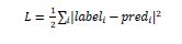
gluon.parameter
mxnet.gluon.parameter is a container that holds the parameters i.e. weights of the Blocks.
Methods and their parameters
Following are some of the important methods and their parameters covered by mxnet.gluon.parameter training module −
| Methods and its Parameters | Definition |
|---|---|
| cast(dtype) | This method will cast data and gradient of this Parameter to a new data type. |
| data([ctx]) | This method will return a copy of this parameter on one context. |
| grad([ctx]) | This method will return a gradient buffer for this parameter on one context. |
| initialize([init, ctx, default_init, ]) | This method will initialize parameter and gradient arrays. |
| list_ctx() | This method will return a list of contexts this parameter is initialized on. |
| list_data() | This method will return copies of this parameter on all contexts. It will be done in the same order as creation. |
| list_grad() | This method will return gradient buffers on all contexts. This will be done in the same order as values(). |
| list_row_sparse_data(row_id) | This method will return copies of the row_sparse parameter on all contexts. This will be done in the same order as creation. |
| reset_ctx(ctx) | This method will re-assign Parameter to other contexts. |
| row_sparse_data(row_id) | This method will return a copy of the row_sparse parameter on the same context as row_ids. |
| set_data(data) | This method will set this parameters value on all contexts. |
| var() | This method will return a symbol representing this parameter. |
| zero_grad() | This method will set the gradient buffer on all contexts to 0. |
Implementation Example
In the example below, we will initialize parameters and the gradients arrays by using initialize() method as follows −
weight = mx.gluon.Parameter('weight', shape=(2, 2))
weight.initialize(ctx=mx.cpu(0))
weight.data()
Output
The output is mentioned below −
[[-0.0256899 0.06511251]
[-0.00243821 -0.00123186]]
<NDArray 2x2 @cpu(0)>
Example
weight.grad()
Output
The output is given below −
[[0. 0.]
[0. 0.]]
<NDArray 2x2 @cpu(0)>
Example
weight.initialize(ctx=[mx.gpu(0), mx.gpu(1)])
weight.data(mx.gpu(0))
Output
You will see the following output −
[[-0.00873779 -0.02834515]
 [ 0.05484822 -0.06206018]]
<NDArray 2x2 @gpu(0)>
Example
weight.data(mx.gpu(1))
Output
When you execute the above code, you should see the following output −
[[-0.00873779 -0.02834515]
 [ 0.05484822 -0.06206018]]
<NDArray 2x2 @gpu(1)>
gluon.trainer
mxnet.gluon.trainer applies an Optimizer on a set of parameters. It should be used together with autograd.
Methods and their parameters
Following are some of the important methods and their parameters covered by mxnet.gluon.trainer training module −
| Methods and its Parameters | Definition |
|---|---|
| allreduce_grads() | This method will reduce the gradients from different contexts for each parameter (weight). |
| load_states(fname) | As name implies, this method will load trainer states. |
| save_states(fname) | As name implies, this method will save trainer states. |
| set_learning_rate(lr) | This method will set a new learning rate of the optimizer. |
| step(batch_size[, ignore_stale_grad]) | This method will make one step of parameter update. It should be called after autograd.backward() and outside of record() scope. |
| update(batch_size[, ignore_stale_grad]) | This method will also make one step of parameter update. It should be called after autograd.backward() and outside of record() scope and after trainer.update(). |
Data Modules
The data modules of Gluon are explained below −
gluon.data
Gluon provides a large number of build-in dataset utilities in gluon.data module. That is the reason it is called the data module.
Classes and their parameters
Following are some of the important methods and their parameters covered by mxnet.gluon.data core module. These methods are typically related to Datasets, Sampling, and DataLoader.
| Methods and its Parameters | Definition |
|---|---|
| ArrayDataset(*args) | This method represents a dataset which combines two or more than two dataset-like objects. For example, Datasets, lists, arrays, etc. |
| BatchSampler(sampler, batch_size[, last_batch]) | This method wraps over another Sampler. Once wrapped it returns the mini batches of samples. |
| DataLoader(dataset[, batch_size, shuffle, ]) | Similar to BatchSampler but this method loads data from a dataset. Once loaded it returns the mini batches of data. |
| This represents the abstract dataset class. | |
| FilterSampler(fn, dataset) | This method represents the samples elements from a Dataset for which fn (function) returns True. |
| RandomSampler(length) | This method represents samples elements from [0, length) randomly without replacement. |
| RecordFileDataset(filename) | It represents a dataset wrapping over a RecordIO file. The extension of the file is .rec. |
| Sampler | This is the base class for samplers. |
| SequentialSampler(length[, start]) | It represents the sample elements from the set [start, start+length) sequentially. |
| It represents the sample elements from the set [start, start+length) sequentially. | This represents the simple Dataset wrapper especially for lists and arrays. |
Implementation Examples
In the example below, we are going to use gluon.data.BatchSampler() API, which wraps over another sampler. It returns the mini batches of samples.
import mxnet as mx
from mxnet.gluon import data
sampler = mx.gluon.data.SequentialSampler(15)
batch_sampler = mx.gluon.data.BatchSampler(sampler, 4, 'keep')
list(batch_sampler)
Output
The output is mentioned below −
[[0, 1, 2, 3], [4, 5, 6, 7], [8, 9, 10, 11], [12, 13, 14]]
gluon.data.vision.datasets
Gluon provides a large number of pre-defined vision dataset functions in gluon.data.vision.datasets module.
Classes and their parameters
MXNet provides us useful and important datasets, whose classes and parameters are given below −
| Classes and its Parameters | Definition |
|---|---|
| MNIST([root, train, transform]) | This is a useful dataset providing us the handwritten digits. The url for MNIST dataset is http://yann.lecun.com/exdb/mnist |
| FashionMNIST([root, train, transform]) | This dataset consists of Zalandos article images consisting of fashion products. It is a drop-in replacement of original MNIST dataset. You can get this dataset from https://github.com/zalandoresearch/fashion-mnist |
| CIFAR10([root, train, transform]) | This is an image classification dataset from https://www.cs.toronto.edu/~kriz/cifar.html. In this dataset each sample is an image with shape (32, 32, 3). |
| CIFAR100([root, fine_label, train, transform]) | This is CIFAR100 image classification dataset from https://www.cs.toronto.edu/~kriz/cifar.html. It also has each sample is an image with shape (32, 32, 3). |
| ImageRecordDataset (filename[, flag, transform]) | This dataset is wrapping over a RecordIO file that contains images. In this each sample is an image with its corresponding label. |
| ImageFolderDataset (root[, flag, transform]) | This is a dataset for loading image files that are stored in a folder structure. |
| ImageListDataset ([root, imglist, flag]) | This is a dataset for loading image files that are specified by a list of entries. |
Example
In the example below, we are going to show the use of ImageListDataset(), which is used for loading image files that are specified by a list of entries −
# written to text file *.lst

0 0 root/cat/0001.jpg
1 0 root/cat/xxxa.jpg
2 0 root/cat/yyyb.jpg
3 1 root/dog/123.jpg
4 1 root/dog/023.jpg
5 1 root/dog/wwww.jpg

# A pure list, each item is a list [imagelabel: float or list of float, imgpath]

[[0, root/cat/0001.jpg]
[0, root/cat/xxxa.jpg]
[0, root/cat/yyyb.jpg]
[1, root/dog/123.jpg]
[1, root/dog/023.jpg]
[1, root/dog/wwww.jpg]]
Utility Modules
The utility modules in Gluon are as follows −
gluon.utils
Gluon provides a large number of build-in parallelisation utility optimiser in gluon.utils module. It provides variety of utilities for training. That is the reason it is called the utility module.
Functions and their parameters
Following are the functions and their parameters consisting in this utility module named gluon.utils −
| Functions and its Parameters | Definition |
|---|---|
| split_data(data, num_slice[, batch_axis, ]) | This function is usually use for data parallelism and each slice is sent to one device i.e. GPU. It splits an NDArray into num_slice slices along batch_axis. |
| split_and_load(data, ctx_list[, batch_axis, ]) | This function splits an NDArray into len(ctx_list) slices along batch_axis. The only difference from above split_data () function is that, it also loads each slice to one context in ctx_list. |
| clip_global_norm(arrays, max_norm[, ]) | The job of this function is to rescale NDArrays in such a way that the sum of their 2-norm is smaller than max_norm. |
| check_sha1(filename, sha1_hash) | This function will check whether the sha1 hash of the file content matches the expected hash or not. |
| download(url[, path, overwrite, sha1_hash, ]) | As name specifies, this function will download a given URL. |
| replace_file(src, dst) | This function will implement atomic os.replace. it will be done with Linux and OSX. |
Python API Autograd and Initializer
This chapter deals with the autograd and initializer API in MXNet.
mxnet.autograd
This is MXNet autograd API for NDArray. It has the following class −
Class: Function()
It is used for customised differentiation in autograd. It can be written as mxnet.autograd.Function. If, for any reason, the user do not want to use the gradients that are computed by the default chain-rule, then he/she can use Function class of mxnet.autograd to customize differentiation for computation. It has two methods namely Forward() and Backward().
Let us understand the working of this class with the help of following points −
First, we need to define our computation in the forward method.
Then, we need to provide the customized differentiation in the backward method.
Now during gradient computation, instead of user-defined backward function, mxnet.autograd will use the backward function defined by the user. We can also cast to numpy array and back for some operations in forward as well as backward.
Example
Before using the mxnet.autograd.function class, lets define a stable sigmoid function with backward as well as forward methods as follows −
class sigmoid(mx.autograd.Function):
   def forward(self, x):
      y = 1 / (1 + mx.nd.exp(-x))
      self.save_for_backward(y)
      return y

   def backward(self, dy):
      y, = self.saved_tensors
      return dy * y * (1-y)
Now, the function class can be used as follows −
func = sigmoid()
x = mx.nd.random.uniform(shape=(10,))
x.attach_grad()
with mx.autograd.record():
m = func(x)
m.backward()
dx_grad = x.grad.asnumpy()
dx_grad
Output
When you run the code, you will see the following output −
array([0.21458015, 0.21291625, 0.23330082, 0.2361367 , 0.23086983,
0.24060014, 0.20326573, 0.21093895, 0.24968489, 0.24301809],
dtype=float32)
Methods and their parameters
Following are the methods and their parameters of mxnet.autogard.function class −
| Methods and its Parameters | Definition |
|---|---|
| forward (heads[, head_grads, retain_graph, ]) | This method is used for forward computation. |
| backward(heads[, head_grads, retain_graph, ]) | This method is used for backward computation. It computes the gradients of heads with respect to previously marked variables. This method takes as many inputs as forwards output. It also returns as many NDArrays as forwards inputs. |
| get_symbol(x) | This method is used to retrieve recorded computation history as Symbol. |
| grad(heads, variables[, head_grads, ]) | This method computes the gradients of heads with respect to variables. Once computed, instead of storing into variable.grad, gradients will be returned as new NDArrays. |
| is_recording() | With the help of this method we can get status on recording and not recording. |
| is_training() | With the help of this method we can get status on training and predicting. |
| mark_variables(variables, gradients[, grad_reqs]) | This method will mark NDArrays as variables to compute gradient for autograd. This method is same as function .attach_grad() in a variable but the only difference is that with this call we can set the gradient to any value. |
| pause([train_mode]) | This method returns a scope context to be used in with statement for codes which do not need gradients to be calculated. |
| predict_mode() | This method returns a scope context to be used in with statement in which forward pass behavior is set to inference mode and that is without changing the recording states. |
| record([train_mode]) | It will return an autograd recording scope context to be used in with statement and captures code which needs gradients to be calculated. |
| set_recording(is_recording) | Similar to is_recoring(), with the help of this method we can get status on recording and not recording. |
| set_training(is_training) | Similar to is_traininig(), with the help of this method we can set status to training or predicting. |
| train_mode() | This method will return a scope context to be used in with statement in which forward pass behavior is set to training mode and that is without changing the recording states. |
Implementation Example
In the below example, we will be using mxnet.autograd.grad() method to compute the gradient of head with respect to variables −
x = mx.nd.ones((2,))
x.attach_grad()
with mx.autograd.record():
z = mx.nd.elemwise_add(mx.nd.exp(x), x)
dx_grad = mx.autograd.grad(z, [x], create_graph=True)
dx_grad
Output
The output is mentioned below −
[
[3.7182817 3.7182817]
<NDArray 2 @cpu(0)>]
We can use mxnet.autograd.predict_mode() method to return a scope to be used in with statement −
with mx.autograd.record():
y = model(x)
with mx.autograd.predict_mode():
y = sampling(y)
backward([y])
mxnet.intializer
This is MXNet API for weigh initializer. It has the following classes −
Classes and their parameters
Following are the methods and their parameters of mxnet.autogard.function class:
| Classes and its Parameters | Definition |
|---|---|
| Bilinear() | With the help of this class we can initialize weight for up-sampling layers. |
| Constant(value) | This class initializes the weights to a given value. The value can be a scalar as well as NDArray that matches the shape of the parameter to be set. |
| FusedRNN(init, num_hidden, num_layers, mode) | As name implies, this class initialize parameters for the fused Recurrent Neural Network (RNN) layers. |
| InitDesc | It acts as the descriptor for the initialization pattern. |
| Initializer(**kwargs) | This is the base class of an initializer. |
| LSTMBias([forget_bias]) | This class initialize all biases of an LSTMCell to 0.0 but except for the forget gate whose bias is set to a custom value. |
| Load(param[, default_init, verbose]) | This class initialize the variables by loading data from file or dictionary. |
| MSRAPrelu([factor_type, slope]) | As name implies, this class Initialize the weight according to a MSRA paper. |
| Mixed(patterns, initializers) | It initializes the parameters using multiple initializers. |
| Normal([sigma]) | Normal() class initializes weights with random values sampled from a normal distribution with a mean of zero and standard deviation (SD) of sigma. |
| One() | It initializes the weights of parameter to one. |
| Orthogonal([scale, rand_type]) | As name implies, this class initialize weight as orthogonal matrix. |
| Uniform([scale]) | It initializes weights with random values which is uniformly sampled from a given range. |
| Xavier([rnd_type, factor_type, magnitude]) | It actually returns an initializer that performs Xavier initialization for weights. |
| Zero() | It initializes the weights of parameter to zero. |
Implementation Example
In the below example, we will be using mxnet.init.Normal() class create an initializer and retrieve its parameters −
init = mx.init.Normal(0.8)
init.dumps()
Output
The output is given below −
'["normal", {"sigma": 0.8}]'
Example
init = mx.init.Xavier(factor_type="in", magnitude=2.45)
init.dumps()
Output
The output is shown below −
'["xavier", {"rnd_type": "uniform", "factor_type": "in", "magnitude": 2.45}]'
In the below example, we will be using mxnet.initializer.Mixed() class to initialize parameters using multiple initializers −
init = mx.initializer.Mixed(['bias', '.*'], [mx.init.Zero(),
mx.init.Uniform(0.1)])
module.init_params(init)

for dictionary in module.get_params():
for key in dictionary:
print(key)
print(dictionary[key].asnumpy())
Output
The output is shown below −
fullyconnected1_weight
[[ 0.0097627 0.01856892 0.04303787]]
fullyconnected1_bias
[ 0.]
Apache MXNet - Python API Symbol
In this chapter, we will learn about an interface in MXNet which is termed as Symbol.
Mxnet.ndarray
Apache MXNets Symbol API is an interface for symbolic programming. Symbol API features the use of the following −
Computational graphs
Reduced memory usage
Pre-use function optimization
The example given below shows how one can create a simple expression by using MXNets Symbol API −
An NDArray by using 1-D and 2-D array from a regular Python list −
import mxnet as mx
# Two placeholders namely x and y will be created with mx.sym.variable
x = mx.sym.Variable('x')
y = mx.sym.Variable('y')
# The symbol here is constructed using the plus + operator.
z = x + y
Output
You will see the following output −
<Symbol _plus0>
Example
(x, y, z)
Output
The output is given below −
(<Symbol x>, <Symbol y>, <Symbol _plus0>)
Now let us discuss in detail about the classes, functions, and parameters of ndarray API of MXNet.
Classes
Following table consists of the classes of Symbol API of MXNet −
| Class | Definition |
|---|---|
| Symbol(handle) | This class namely symbol is the symbolic graph of the Apache MXNet. |
Functions and their parameters
Following are some of the important functions and their parameters covered by mxnet.Symbol API −
| Function and its Parameters | Definition |
|---|---|
| Activation([data, act_type, out, name]) | It applies an activation function element-wise to the input. It supports relu, sigmoid, tanh, softrelu, softsign activation functions. |
| BatchNorm([data, gamma, beta, moving_mean, ]) | It is used for batch normalization. This function normalizes a data batch by mean and variance. It applies a scale gamma and offset beta. |
| BilinearSampler([data, grid, cudnn_off, ]) | This function applies bilinear sampling to input feature map. Actually it is the key of Spatial Transformer Networks. If you are familiar with remap function in OpenCV, the usage of this function is quite similar to that. The only difference is that it has the backward pass. |
| BlockGrad([data, out, name]) | As name specifies, this function stops gradient computation. It basically stops the accumulated gradient of the inputs from flowing through this operator in backward direction. |
| cast([data, dtype, out, name]) | This function will cast all elements of the input to a new type. |
| This function will cast all elements of the input to a new type. | This function, as name specified, returns a new symbol of given shape and type, filled with zeros. |
| ones(shape[, dtype]) | This function, as name specified return a new symbol of given shape and type, filled with ones. |
| full(shape, val[, dtype]) | This function, as name specified returns a new array of given shape and type, filled with the given value val. |
| arange(start[, stop, step, repeat, ]) | It will return evenly spaced values within a given interval. The values are generated within half open interval [start, stop) which means that the interval includes start but excludes stop. |
| linspace(start, stop, num[, endpoint, name, ]) | It will return evenly spaced numbers within a specified interval. Similar to the function arrange(), the values are generated within half open interval [start, stop) which means that the interval includes start but excludes stop. |
| histogram(a[, bins, range]) | As name implies, this function will compute the histogram of the input data. |
| power(base, exp) | As name implies, this function will return element-wise result of base element raised to powers from exp element. Both inputs i.e. base and exp, can be either Symbol or scalar. Here note that broadcasting is not allowed. You can use broadcast_pow if you want to use the feature of broadcast. |
| SoftmaxActivation([data, mode, name, attr, out]) | This function applies softmax activation to input. It is intended for internal layers. It is actually deprecated, we can use softmax() instead. |
Implementation Examples
In the example below we will be using the function power() which will return element-wise result of base element raised to the powers from exp element:
import mxnet as mx mx.sym.power(3, 5)
Output
You will see the following output −
243
Example
x = mx.sym.Variable('x')
y = mx.sym.Variable('y')
z = mx.sym.power(x, 3)
z.eval(x=mx.nd.array([1,2]))[0].asnumpy()
Output
This produces the following output −
array([1., 8.], dtype=float32)
Example
z = mx.sym.power(4, y) z.eval(y=mx.nd.array([2,3]))[0].asnumpy()
Output
When you execute the above code, you should see the following output −
array([16., 64.], dtype=float32)
Example
z = mx.sym.power(x, y) z.eval(x=mx.nd.array([4,5]), y=mx.nd.array([2,3]))[0].asnumpy()
Output
The output is mentioned below −
array([ 16., 125.], dtype=float32)
In the example given below, we will be using the function SoftmaxActivation() (or softmax()) which will be applied to input and is intended for internal layers.
input_data = mx.nd.array([[2., 0.9, -0.5, 4., 8.], [4., -.7, 9., 2., 0.9]]) soft_max_act = mx.nd.softmax(input_data) print (soft_max_act.asnumpy())
Output
You will see the following output −
[[2.4258138e-03 8.0748333e-04 1.9912292e-04 1.7924475e-02 9.7864312e-01] [6.6843745e-03 6.0796250e-05 9.9204916e-01 9.0463174e-04 3.0112563e-04]]
symbol.contrib
The Contrib NDArray API is defined in the symbol.contrib package. It typically provides many useful experimental APIs for new features. This API works as a place for the community where they can try out the new features. The feature contributor will get the feedback as well.
Functions and their parameters
Following are some of the important functions and their parameters covered by mxnet.symbol.contrib API −
| Function and its Parameters | Definition |
|---|---|
| rand_zipfian(true_classes, num_sampled, ) | This function draws random samples from an approximately Zipfian distribution. The base distribution of this function is Zipfian distribution. This function randomly samples num_sampled candidates and the elements of sampled_candidates are drawn from the base distribution given above. |
| foreach(body, data, init_states) | As name implies, this function runs a loop with user-defined computation over NDArrays on dimension 0. This function simulates a for loop and body has the computation for an iteration of the for loop. |
| while_loop(cond, func, loop_vars[, ]) | As name implies, this function runs a while loop with user-defined computation and loop condition. This function simulates a while loop that literately does customized computation if the condition is satisfied. |
| cond(pred, then_func, else_func) | As name implies, this function run an if-then-else using user-defined condition and computation. This function simulates an if-like branch which chooses to do one of the two customized computations according to the specified condition. |
| getnnz([data, axis, out, name]) | This function gives us the number of stored values for a sparse tensor. It also includes explicit zeros. It only supports CSR matrix on CPU. |
| requantize([data, min_range, max_range, ]) | This function requantize the given data that is quantized in int32 and the corresponding thresholds, into int8 using min and max thresholds either calculated at runtime or from calibration. |
| index_copy([old_tensor, index_vector, ]) | This function copies the elements of a new_tensor into the old_tensor by selecting the indices in the order given in index. The output of this operator will be a new tensor that contains the rest elements of old tensor and the copied elements of new tensor. |
| interleaved_matmul_encdec_qk([queries, ]) | This operator compute the matrix multiplication between the projections of queries and keys in multi-head attention use as encoder-decoder. The condition is that the inputs should be a tensor of projections of queries that follows the layout: (seq_length, batch_size, num_heads*, head_dim). |
Implementation Examples
In the example below we will be using the function rand_zipfian for drawing random samples from an approximately Zipfian distribution −
import mxnet as mx
true_cls = mx.sym.Variable('true_cls')
samples, exp_count_true, exp_count_sample = mx.sym.contrib.rand_zipfian(true_cls, 5, 6)
samples.eval(true_cls=mx.nd.array([3]))[0].asnumpy()
Output
You will see the following output −
array([4, 0, 2, 1, 5], dtype=int64)
Example
exp_count_true.eval(true_cls=mx.nd.array([3]))[0].asnumpy()
Output
The output is mentioned below −
array([0.57336551])
Example
exp_count_sample.eval(true_cls=mx.nd.array([3]))[0].asnumpy()
Output
You will see the following output −
array([1.78103594, 0.46847373, 1.04183923, 0.57336551, 1.04183923])
In the example below we will be using the function while_loop for running a while loop for user-defined computation and loop condition −
cond = lambda i, s: i <= 7
func = lambda i, s: ([i + s], [i + 1, s + i])
loop_vars = (mx.sym.var('i'), mx.sym.var('s'))
outputs, states = mx.sym.contrib.while_loop(cond, func, loop_vars, max_iterations=10)
print(outputs)
Output
The output is given below:
[<Symbol _while_loop0>]
Example
Print(States)
Output
This produces the following output −
[<Symbol _while_loop0>, <Symbol _while_loop0>]
In the example below we will be using the function index_copy that copies the elements of new_tensor into the old_tensor.
import mxnet as mx a = mx.nd.zeros((6,3)) b = mx.nd.array([[1,2,3],[4,5,6],[7,8,9]]) index = mx.nd.array([0,4,2]) mx.nd.contrib.index_copy(a, index, b)
Output
When you execute the above code, you should see the following output −
[[1. 2. 3.] [0. 0. 0.] [7. 8. 9.] [0. 0. 0.] [4. 5. 6.] [0. 0. 0.]] <NDArray 6x3 @cpu(0)>
symbol.image
The Image Symbol API is defined in the symbol.image package. As name implies, it typically used for images and their features.
Functions and their parameters
Following are some of the important functions and their parameters covered by mxnet.symbol.image API −
| Function and its Parameters | Definition |
|---|---|
| adjust_lighting([data, alpha, out, name]) | As name implies, this function adjusts the lighting level of the input. It follows the AlexNet style. |
| crop([data, x, y, width, height, out, name]) | With the help of this function we can crop an image NDArray of shape (H x W x C) or (N x H x W x C) to the size given by user. |
| normalize([data, mean, std, out, name]) | It will normalize an tensor of shape (C x H x W) or (N x C x H x W) with mean and standard deviation(SD). |
| random_crop([data, xrange, yrange, width, ]) | Similar to crop(), it randomly crop an image NDArray of shape (H x W x C) or (N x H x W x C) to the size given by the user. It will upsample the result if src is smaller than the size. |
| random_lighting([data, alpha_std, out, name]) | As name implies, this function adds the PCA noise randomly. It also follows the AlexNet style. |
| random_resized_crop([data, xrange, yrange, ]) | It also crops an image randomly NDArray of shape (H x W x C) or (N x H x W x C) to the given size. It will upsample the result if src is smaller than the size. It will randomize the area and aspect ration as well. |
| resize([data, size, keep_ratio, interp, ]) | As name implies, this function will resize an image NDArray of shape (H x W x C) or (N x H x W x C) to the size given by user. |
| to_tensor([data, out, name]) | It converts an image NDArray of shape (H x W x C) or (N x H x W x C) with the values in the range [0, 255] to a tensor NDArray of shape (C x H x W) or (N x C x H x W) with the values in the range [0, 1]. |
Implementation Examples
In the example below, we will be using the function to_tensor to convert image NDArray of shape (H x W x C) or (N x H x W x C) with the values in the range [0, 255] to a tensor NDArray of shape (C x H x W) or (N x C x H x W) with the values in the range [0, 1].
import numpy as np img = mx.sym.random.uniform(0, 255, (4, 2, 3)).astype(dtype=np.uint8) mx.sym.image.to_tensor(img)
Output
The output is stated below −
<Symbol to_tensor4>
Example
img = mx.sym.random.uniform(0, 255, (2, 4, 2, 3)).astype(dtype=np.uint8) mx.sym.image.to_tensor(img)
Output
The output is mentioned below:
<Symbol to_tensor5>
In the example below, we will be using the function normalize() to normalize an tensor of shape (C x H x W) or (N x C x H x W) with mean and standard deviation(SD).
img = mx.sym.random.uniform(0, 1, (3, 4, 2)) mx.sym.image.normalize(img, mean=(0, 1, 2), std=(3, 2, 1))
Output
Given below is the output of the code −
<Symbol normalize0>
Example
img = mx.sym.random.uniform(0, 1, (2, 3, 4, 2)) mx.sym.image.normalize(img, mean=(0, 1, 2), std=(3, 2, 1))
Output
The output is shown below −
<Symbol normalize1>
symbol.random
The Random Symbol API is defined in the symbol.random package. As name implies, it is random distribution generator Symbol API of MXNet.
Functions and their parameters
Following are some of the important functions and their parameters covered by mxnet.symbol.random API −
| Function and its Parameters | Definition |
|---|---|
| uniform([low, high, shape, dtype, ctx, out]) | It generates random samples from a uniform distribution. |
| normal([loc, scale, shape, dtype, ctx, out]) | It generates random samples from a normal (Gaussian) distribution. |
| randn(*shape, **kwargs) | It generates random samples from a normal (Gaussian) distribution. |
| poisson([lam, shape, dtype, ctx, out]) | It generates random samples from a Poisson distribution. |
| exponential([scale, shape, dtype, ctx, out]) | It generates samples from an exponential distribution. |
| gamma([alpha, beta, shape, dtype, ctx, out]) | It generates random samples from a gamma distribution. |
| multinomial(data[, shape, get_prob, out, dtype]) | It generates concurrent sampling from multiple multinomial distributions. |
| negative_binomial([k, p, shape, dtype, ctx, out]) | It generates random samples from a negative binomial distribution. |
| generalized_negative_binomial([mu, alpha, ]) | It generates random samples from a generalized negative binomial distribution. |
| shuffle(data, **kwargs) | It shuffles the elements randomly. |
| randint(low, high[, shape, dtype, ctx, out]) | It generates random samples from a discrete uniform distribution. |
| exponential_like([data, lam, out, name]) | It generates random samples from an exponential distribution according to the input array shape. |
| gamma_like([data, alpha, beta, out, name]) | It generates random samples from a gamma distribution according to the input array shape. |
| generalized_negative_binomial_like([data, ]) | It generates random samples from a generalized negative binomial distribution according to the input array shape. |
| negative_binomial_like([data, k, p, out, name]) | It generates random samples from a negative binomial distribution according to the input array shape. |
| normal_like([data, loc, scale, out, name]) | It generates random samples from a normal (Gaussian) distribution according to the input array shape. |
| poisson_like([data, lam, out, name]) | It generates random samples from a Poisson distribution according to the input array shape. |
| uniform_like([data, low, high, out, name]) | It generates random samples from a uniform distribution according to the input array shape. |
Implementation Examples
In the example below, we are going to shuffle the elements randomly using shuffle() function. It will shuffle the array along the first axis.
data = mx.nd.array([[0, 1, 2], [3, 4, 5], [6, 7, 8],[9,10,11]])
x = mx.sym.Variable('x')
y = mx.sym.random.shuffle(x)
y.eval(x=data)
Output
You will see the following output:
[ [[ 9. 10. 11.] [ 0. 1. 2.] [ 6. 7. 8.] [ 3. 4. 5.]] <NDArray 4x3 @cpu(0)>]
Example
y.eval(x=data)
Output
When you execute the above code, you should see the following output −
[ [[ 6. 7. 8.] [ 0. 1. 2.] [ 3. 4. 5.] [ 9. 10. 11.]] <NDArray 4x3 @cpu(0)>]
In the example below, we are going to draw random samples from a generalized negative binomial distribution. For this will be using the function generalized_negative_binomial().
mx.sym.random.generalized_negative_binomial(10, 0.1)
Output
The output is given below −
<Symbol _random_generalized_negative_binomial0>
symbol.sparse
The Sparse Symbol API is defined in the mxnet.symbol.sparse package. As name implies, it provides sparse neural network graphs and auto-differentiation on CPU.
Functions and their parameters
Following are some of the important functions (includes Symbol creation routines, Symbol Manipulation routines, Mathematical functions, Trigonometric function, Hyberbolic functions, Reduce functions, Rounding, Powers, Neural Network) and their parameters covered by mxnet.symbol.sparse API −
| Function and its Parameters | Definition |
|---|---|
| ElementWiseSum(*args, **kwargs) | This function will add all input arguments element wise. For example, _(1,2,=1+2++). Here, we can see that add_n is potentially more efficient than calling add by n times. |
| Embedding([data, weight, input_dim, ]) | It will map the integer indices to vector representations i.e. embeddings. It actually maps words to real-valued vectors in high-dimensional space which is called word embeddings. |
| LinearRegressionOutput([data, label, ]) | It computes and optimizes for squared loss during backward propagation giving just output data during forward propagation. |
| LogisticRegressionOutput([data, label, ]) | Applies a logistic function which is also called the sigmoid function to the input. The function is computed as 1/1+exp (−x). |
| MAERegressionOutput([data, label, ]) | This operator computes mean absolute error of the input. MAE is actually a risk metric corresponding to the expected value of absolute error. |
| abs([data, name, attr, out]) | As name implies, this function will return element-wise absolute value of the input. |
| adagrad_update([weight, grad, history, lr, ]) | It is an update function for AdaGrad optimizer. |
| adam_update([weight, grad, mean, var, lr, ]) | It is an update function for Adam optimizer. |
| add_n(*args, **kwargs) | As name implies it will adds all input arguments element-wise. |
| arccos([data, name, attr, out]) | This function will returns element-wise inverse cosine of the input array. |
| dot([lhs, rhs, transpose_a, transpose_b, ]) | As name implies, it will give the dot product of two arrays. It will depend upon the input array dimension: 1-D: inner product of vectors 2-D: matrix multiplication N-D: A sum product over the last axis of the first input and the first axis of the second input. |
| elemwise_add([lhs, rhs, name, attr, out]) | As name implies it will add arguments element wise. |
| elemwise_div([lhs, rhs, name, attr, out]) | As name implies it will divide arguments element wise. |
| elemwise_mul([lhs, rhs, name, attr, out]) | As name implies it will Multiply arguments element wise. |
| elemwise_sub([lhs, rhs, name, attr, out]) | As name implies it will Subtract arguments element wise. |
| exp([data, name, attr, out]) | This function will return element wise exponential value of the given input. |
| sgd_update([weight, grad, lr, wd, ]) | It acts as an update function for Stochastic Gradient Descent optimizer. |
| sigmoid([data, name, attr, out]) | As name implies it will compute sigmoid of x element wise. |
| sign([data, name, attr, out]) | It will return the element wise sign of the given input. |
| sin([data, name, attr, out]) | As name implies, this function will computes the element wise sine of the given input array. |
Implementation Example
In the example below, we are going to shuffle the elements randomly using ElementWiseSum() function. It will map integer indices to vector representations i.e. word embeddings.
input_dim = 4 output_dim = 5
Example
/* Here every row in weight matrix y represents a word. So, y = (w0,w1,w2,w3) y = [[ 0., 1., 2., 3., 4.], [ 5., 6., 7., 8., 9.], [ 10., 11., 12., 13., 14.], [ 15., 16., 17., 18., 19.]] /* Here input array x represents n-grams(2-gram). So, x = [(w1,w3), (w0,w2)] x = [[ 1., 3.], [ 0., 2.]] /* Now, Mapped input x to its vector representation y. Embedding(x, y, 4, 5) = [[[ 5., 6., 7., 8., 9.], [ 15., 16., 17., 18., 19.]], [[ 0., 1., 2., 3., 4.], [ 10., 11., 12., 13., 14.]]]
Apache MXNet - Python API Module
Apache MXNets module API is like a FeedForward model and it is easier to compose similar to Torch module. It consists of following classes −
BaseModule([logger])
It represents the base class of a module. A module can be thought of as computation component or computation machine. The job of a module is to execute forward and backward passes. It also updates parameters in a model.
Methods
Following table shows the methods consisted in BaseModule class−
| Methods | Definition |
|---|---|
| backward([out_grads]) | As name implies this method implements the backward computation. |
| bind(data_shapes[, label_shapes, ]) | It binds the symbols to construct executors and it is necessary before one can perform computation with the module. |
| fit(train_data[, eval_data, eval_metric, ]) | This method trains the module parameters. |
| forward(data_batch[, is_train]) | As name implies this method implements the Forward computation. This method supports data batches with various shapes like different batch sizes or different image sizes. |
| forward_backward(data_batch) | It is a convenient function, as name implies, that calls both forward and backward. |
| get_input_grads([merge_multi_context]) | This method will gets the gradients to the inputs which is computed in the previous backward computation. |
| get_outputs([merge_multi_context]) | As name implies, this method will gets outputs of the previous forward computation. |
| get_params() | It gets the parameters especially those which are potentially copies of the actual parameters used to do computation on the device. |
| get_states([merge_multi_context]) | This method will get states from all devices |
| init_optimizer([kvstore, optimizer, ]) | This method installs and initialize the optimizers. It also initializes kvstore for distribute training. |
| init_params([initializer, arg_params, ]) | As name implies, this method will initialize the parameters and auxiliary states. |
| install_monitor(mon) | This method will install monitor on all executors. |
| iter_predict(eval_data[, num_batch, reset, ]) | This method will iterate over predictions. |
| load_params(fname) | It will, as name specifies, load model parameters from file. |
| predict(eval_data[, num_batch, ]) | It will run the prediction and collects the outputs as well. |
| prepare(data_batch[, sparse_row_id_fn]) | The operator prepares the module for processing a given data batch. |
| save_params(fname) | As name specifies, this function will save the model parameters to file. |
| score(eval_data, eval_metric[, num_batch, ]) | It runs the prediction on eval_data and also evaluates the performance according to the given eval_metric. |
| set_params(arg_params, aux_params[, ]) | This method will assign the parameter and aux state values. |
| set_states([states, value]) | This method, as name implies, sets value for states. |
| update() | This method updates the given parameters according to the installed optimizer. It also updates the gradients computed in the previous forward-backward batch. |
| update_metric(eval_metric, labels[, pre_sliced]) | This method, as name implies, evaluates and accumulates the evaluation metric on outputs of the last forward computation. |
| backward([out_grads]) | As name implies this method implements the backward computation. |
| bind(data_shapes[, label_shapes, ]) | It set up the buckets and binds the executor for the default bucket key. This method represents the binding for a BucketingModule. |
| forward(data_batch[, is_train]) | As name implies this method implements the Forward computation. This method supports data batches with various shapes like different batch sizes or different image sizes. |
| get_input_grads([merge_multi_context]) | This method will get the gradients to the inputs which is computed in the previous backward computation. |
| get_outputs([merge_multi_context]) | As name implies, this method will get outputs from the previous forward computation. |
| get_params() | It gets the current parameters especially those which are potentially copies of the actual parameters used to do computation on the device. |
| get_states([merge_multi_context]) | This method will get states from all devices. |
| init_optimizer([kvstore, optimizer, ]) | This method installs and initialize the optimizers. It also initializes kvstore for distribute training. |
| init_params([initializer, arg_params, ]) | As name implies, this method will initialize the parameters and auxiliary states. |
| install_monitor(mon) | This method will install monitor on all executors. |
| load(prefix, epoch[, sym_gen, ]) | This method will create a model from the previously saved checkpoint. |
| load_dict([sym_dict, sym_gen, ]) | This method will create a model from a dictionary (dict) mapping bucket_key to symbols. It also shares arg_params and aux_params. |
| prepare(data_batch[, sparse_row_id_fn]) | The operator prepares the module for processing a given data batch. |
| save_checkpoint(prefix, epoch[, remove_amp_cast]) | This method, as name implies, saves the current progress to the checkpoint for all buckets in BucketingModule. It is recommended to use mx.callback.module_checkpoint as epoch_end_callback to save during training. |
| set_params(arg_params, aux_params[,]) | As name specifies, this function will assign parameters and aux state values. |
| set_states([states, value]) | This method, as name implies, sets value for states. |
| switch_bucket(bucket_key, data_shapes[, ]) | It will switche to a different bucket. |
| update() | This method updates the given parameters according to the installed optimizer. It also updates the gradients computed in the previous forward-backward batch. |
| update_metric(eval_metric, labels[, pre_sliced]) | This method, as name implies, evaluates and accumulates the evaluation metric on outputs of the last forward computation. |
Attributes
Following table shows the attributes consisted in the methods of BaseModule class −
| Attributes | Definition |
|---|---|
| data_names | It consists of the list of names for data required by this module. |
| data_shapes | It consists of the list of (name, shape) pairs specifying the data inputs to this module. |
| label_shapes | It shows the list of (name, shape) pairs specifying the label inputs to this module. |
| output_names | It consists of the list of names for the outputs of this module. |
| output_shapes | It consists of the list of (name, shape) pairs specifying the outputs of this module. |
| symbol | As name specified, this attribute gets the symbol associated with this module. |
data_shapes: You can refer the link available at https://mxnet.apache.org for details. output_shapes: More
output_shapes: More information is available at https://mxnet.apache.org/api/python
BucketingModule(sym_gen[])
It represents the Bucketingmodule class of a Module which helps to deal efficiently with varying length inputs.
Methods
Following table shows the methods consisted in BucketingModule class −
Attributes
Following table shows the attributes consisted in the methods of BaseModule class −
| Attributes | Definition |
|---|---|
| data_names | It consists of the list of names for data required by this module. |
| data_shapes | It consists of the list of (name, shape) pairs specifying the data inputs to this module. |
| label_shapes | It shows the list of (name, shape) pairs specifying the label inputs to this module. |
| output_names | It consists of the list of names for the outputs of this module. |
| output_shapes | It consists of the list of (name, shape) pairs specifying the outputs of this module. |
| Symbol | As name specified, this attribute gets the symbol associated with this module. |
data_shapes − You can refer the link at https://mxnet.apache.org/api/python/docs for more information.
output_shapes− You can refer the link at https://mxnet.apache.org/api/python/docs for more information.
Module(symbol[,data_names, label_names,])
It represents a basic module that wrap a symbol.
Methods
Following table shows the methods consisted in Module class −
| Methods | Definition |
|---|---|
| backward([out_grads]) | As name implies this method implements the backward computation. |
| bind(data_shapes[, label_shapes, ]) | It binds the symbols to construct executors and it is necessary before one can perform computation with the module. |
| borrow_optimizer(shared_module) | As name implies, this method will borrow the optimizer from a shared module. |
| forward(data_batch[, is_train]) | As name implies this method implements the Forward computation. This method supports data batches with various shapes like different batch sizes or different image sizes. |
| get_input_grads([merge_multi_context]) | This method will gets the gradients to the inputs which is computed in the previous backward computation. |
| get_outputs([merge_multi_context]) | As name implies, this method will gets outputs of the previous forward computation. |
| get_params() | It gets the parameters especially those which are potentially copies of the actual parameters used to do computation on the device. |
| get_states([merge_multi_context]) | This method will get states from all devices |
| init_optimizer([kvstore, optimizer, ]) | This method installs and initialize the optimizers. It also initializes kvstore for distribute training. |
| init_params([initializer, arg_params, ]) | As name implies, this method will initialize the parameters and auxiliary states. |
| install_monitor(mon) | This method will install monitor on all executors. |
| load(prefix, epoch[, sym_gen, ]) | This method will create a model from the previously saved checkpoint. |
| load_optimizer_states(fname) | This method will load an optimizer i.e. the updater state from a file. |
| prepare(data_batch[, sparse_row_id_fn]) | The operator prepares the module for processing a given data batch. |
| reshape(data_shapes[, label_shapes]) | This method, as name implies, reshape the module for new input shapes. |
| save_checkpoint(prefix, epoch[, ]) | It saves the current progress to checkpoint. |
| save_optimizer_states(fname) | This method saves the optimizer or the updater state to a file. |
| set_params(arg_params, aux_params[,]) | As name specifies, this function will assign parameters and aux state values. |
| set_states([states, value]) | This method, as name implies, sets value for states. |
| update() | This method updates the given parameters according to the installed optimizer. It also updates the gradients computed in the previous forward-backward batch. |
| update_metric(eval_metric, labels[, pre_sliced]) | This method, as name implies, evaluates and accumulates the evaluation metric on outputs of the last forward computation. |
Attributes
Following table shows the attributes consisted in the methods of Module class −
| Attributes | Definition |
|---|---|
| data_names | It consists of the list of names for data required by this module. |
| data_shapes | It consists of the list of (name, shape) pairs specifying the data inputs to this module. |
| label_shapes | It shows the list of (name, shape) pairs specifying the label inputs to this module. |
| output_names | It consists of the list of names for the outputs of this module. |
| output_shapes | It consists of the list of (name, shape) pairs specifying the outputs of this module. |
| label_names | It consists of the list of names for labels required by this module. |
data_shapes: Visit the link https://mxnet.apache.org/api/python/docs/api/module for further details.
output_shapes: The link given herewith https://mxnet.apache.org/api/python/docs/api/module/index.html will offer other important information.
PythonLossModule([name,data_names,])
The base of this class is mxnet.module.python_module.PythonModule. PythonLossModule class is a convenient module class which implements all or many of the module APIs as empty functions.
Methods
Following table shows the methods consisted in PythonLossModule class:
| Methods | Definition |
|---|---|
| backward([out_grads]) | As name implies this method implements the backward computation. |
| forward(data_batch[, is_train]) | As name implies this method implements the Forward computation. This method supports data batches with various shapes like different batch sizes or different image sizes. |
| get_input_grads([merge_multi_context]) | This method will gets the gradients to the inputs which is computed in the previous backward computation. |
| get_outputs([merge_multi_context]) | As name implies, this method will gets outputs of the previous forward computation. |
| install_monitor(mon) | This method will install monitor on all executors. |
PythonModule([data_names,label_names])
The base of this class is mxnet.module.base_module.BaseModule. PythonModule class also is a convenient module class which implements all or many of the module APIs as empty functions.
Methods
Following table shows the methods consisted in PythonModule class −
| Methods | Definition |
|---|---|
| bind(data_shapes[, label_shapes, ]) | It binds the symbols to construct executors and it is necessary before one can perform computation with the module. |
| get_params() | It gets the parameters especially those which are potentially copies of the actual parameters used to do computation on the device. |
| init_optimizer([kvstore, optimizer, ]) | This method installs and initialize the optimizers. It also initializes kvstore for distribute training. |
| init_params([initializer, arg_params, ]) | As name implies, this method will initialize the parameters and auxiliary states. |
| update() | This method updates the given parameters according to the installed optimizer. It also updates the gradients computed in the previous forward-backward batch. |
| update_metric(eval_metric, labels[, pre_sliced]) | This method, as name implies, evaluates and accumulates the evaluation metric on outputs of the last forward computation. |
Attributes
Following table shows the attributes consisted in the methods of PythonModule class −
| Attributes | Definition |
|---|---|
| data_names | It consists of the list of names for data required by this module. |
| data_shapes | It consists of the list of (name, shape) pairs specifying the data inputs to this module. |
| label_shapes | It shows the list of (name, shape) pairs specifying the label inputs to this module. |
| output_names | It consists of the list of names for the outputs of this module. |
| output_shapes | It consists of the list of (name, shape) pairs specifying the outputs of this module. |
data_shapes − Follow the link https://mxnet.apache.org for details.
output_shapes − For more details, visit the link available at https://mxnet.apache.org
SequentialModule([logger])
The base of this class is mxnet.module.base_module.BaseModule. SequentialModule class also is a container module that can chain more than two (multiple) modules together.
Methods
Following table shows the methods consisted in SequentialModule class
| Methods | Definition |
|---|---|
| add(module, **kwargs) | This is most important function of this class. It adds a module to the chain. |
| backward([out_grads]) | As name implies this method implements the backward computation. |
| bind(data_shapes[, label_shapes, ]) | It binds the symbols to construct executors and it is necessary before one can perform computation with the module. |
| forward(data_batch[, is_train]) | As name implies this method implements the Forward computation. This method supports data batches with various shapes like different batch sizes or different image sizes. |
| get_input_grads([merge_multi_context]) | This method will gets the gradients to the inputs which is computed in the previous backward computation. |
| get_outputs([merge_multi_context]) | As name implies, this method will gets outputs of the previous forward computation. |
| get_params() | It gets the parameters especially those which are potentially copies of the actual parameters used to do computation on the device. |
| init_optimizer([kvstore, optimizer, ]) | This method installs and initialize the optimizers. It also initializes kvstore for distribute training. |
| init_params([initializer, arg_params, ]) | As name implies, this method will initialize the parameters and auxiliary states. |
| install_monitor(mon) | This method will install monitor on all executors. |
| update() | This method updates the given parameters according to the installed optimizer. It also updates the gradients computed in the previous forward-backward batch. |
| update_metric(eval_metric, labels[, pre_sliced]) | This method, as name implies, evaluates and accumulates the evaluation metric on outputs of the last forward computation. |
Attributes
Following table shows the attributes consisted in the methods of BaseModule class −
| Attributes | Definition |
|---|---|
| data_names | It consists of the list of names for data required by this module. |
| data_shapes | It consists of the list of (name, shape) pairs specifying the data inputs to this module. |
| label_shapes | It shows the list of (name, shape) pairs specifying the label inputs to this module. |
| output_names | It consists of the list of names for the outputs of this module. |
| output_shapes | It consists of the list of (name, shape) pairs specifying the outputs of this module. | output_shapes | It consists of the list of (name, shape) pairs specifying the outputs of this module. |
data_shapes − The link given herewith https://mxnet.apache.org will help you in understanding the attribute in much detail.
output_shapes − Follow the link available at https://mxnet.apache.org/api for details.
Implementation Examples
In the example below, we are going create a mxnet module.
import mxnet as mx
input_data = mx.symbol.Variable('input_data')
f_connected1 = mx.symbol.FullyConnected(data, name='f_connected1', num_hidden=128)
activation_1 = mx.symbol.Activation(f_connected1, name='relu1', act_type="relu")
f_connected2 = mx.symbol.FullyConnected(activation_1, name = 'f_connected2', num_hidden = 64)
activation_2 = mx.symbol.Activation(f_connected2, name='relu2',
act_type="relu")
f_connected3 = mx.symbol.FullyConnected(activation_2, name='fc3', num_hidden=10)
out = mx.symbol.SoftmaxOutput(f_connected3, name = 'softmax')
mod = mx.mod.Module(out)
print(out)
Output
The output is mentioned below −
<Symbol softmax>
Example
print(mod)
Output
The output is shown below −
<mxnet.module.module.Module object at 0x00000123A9892F28>
In this example below, we will be implementing forward computation
import mxnet as mx
from collections import namedtuple
Batch = namedtuple('Batch', ['data'])
data = mx.sym.Variable('data')
out = data * 2
mod = mx.mod.Module(symbol=out, label_names=None)
mod.bind(data_shapes=[('data', (1, 10))])
mod.init_params()
data1 = [mx.nd.ones((1, 10))]
mod.forward(Batch(data1))
print (mod.get_outputs()[0].asnumpy())
Output
When you execute the above code, you should see the following output −
[[2. 2. 2. 2. 2. 2. 2. 2. 2. 2.]]
Example
data2 = [mx.nd.ones((3, 5))] mod.forward(Batch(data2)) print (mod.get_outputs()[0].asnumpy())
Output
Given below is the output of the code −
[[2. 2. 2. 2. 2.] [2. 2. 2. 2. 2.] [2. 2. 2. 2. 2.]]
