- Apache MXNet - Home
- Apache MXNet - Introduction
- Apache MXNet - Installing MXNet
- Apache MXNet - Toolkits and Ecosystem
- Apache MXNet - System Architecture
- Apache MXNet - System Components
- Apache MXNet - Unified Operator API
- Apache MXNet - Distributed Training
- Apache MXNet - Python Packages
- Apache MXNet - NDArray
- Apache MXNet - Gluon
- Apache MXNet - KVStore and Visualization
- Apache MXNet - Python API ndarray
- Apache MXNet - Python API gluon
- Apache MXNet - Python API autograd and initializer
- Apache MXNet - Python API Symbol
- Apache MXNet - Python API Module
- Apache MXNet Useful Resources
- Apache MXNet - Quick Guide
- Apache MXNet - Useful Resources
- Apache MXNet - Discussion
Apache MXNet - Python API gluon
As we have already discussed in previous chapters that, MXNet Gluon provides a clear, concise, and simple API for DL projects. It enables Apache MXNet to prototype, build, and train DL models without forfeiting the training speed.
Core Modules
Let us learn the core modules of Apache MXNet Python application programming interface (API) gluon.
gluon.nn
Gluon provides a large number of build-in NN layers in gluon.nn module. That is the reason it is called the core module.
Methods and their parameters
Following are some of the important methods and their parameters covered by mxnet.gluon.nn core module −
| Methods and its Parameters | Definition |
|---|---|
| Activation(activation, **kwargs) | As name implies, this method applies an activation function to input. |
| AvgPool1D([pool_size, strides, padding, ]) | This is average pooling operation for temporal data. |
| AvgPool2D([pool_size, strides, padding, ]) | This is average pooling operation for spatial data. |
| AvgPool3D([pool_size, strides, padding, ]) | This is Average pooling operation for 3D data. The data can be spatial or spatio-temporal. |
| BatchNorm([axis, momentum, epsilon, center, ]) | It represents batch normalisation layer. |
| BatchNormReLU([axis, momentum, epsilon, ]) | It also represents batch normalisation layer but with Relu activation function. |
| Block([prefix, params]) | It gives the base class for all neural network layers and models. |
| Conv1D(channels, kernel_size[, strides, ]) | This method is used for 1-D convolution layer. For example, temporal convolution. |
| Conv1DTranspose(channels, kernel_size[, ]) | This method is used for Transposed 1D convolution layer. |
| Conv2D(channels, kernel_size[, strides, ]) | This method is used for 2D convolution layer. For example, spatial convolution over images). |
| Conv2DTranspose(channels, kernel_size[, ]) | This method is used for Transposed 2D convolution layer. |
| Conv3D(channels, kernel_size[, strides, ]) | This method is used for 3D convolution layer. For example, spatial convolution over volumes. |
| Conv3DTranspose(channels, kernel_size[, ]) | This method is used for Transposed 3D convolution layer. |
| Dense(units[, activation, use_bias, ]) | This method represents for your regular densely-connected NN layer. |
| Dropout(rate[, axes]) | As name implies, the method applies Dropout to the input. |
| ELU([alpha]) | This method is used for Exponential Linear Unit (ELU). |
| Embedding(input_dim, output_dim[, dtype, ]) | It turns non-negative integers into dense vectors of fixed size. |
| Flatten(**kwargs) | This method flattens the input to 2-D. |
| GELU(**kwargs) | This method is used for Gaussian Exponential Linear Unit (GELU). |
| GlobalAvgPool1D([layout]) | With the help of this method, we can do global average pooling operation for temporal data. |
| GlobalAvgPool2D([layout]) | With the help of this method, we can do global average pooling operation for spatial data. |
| GlobalAvgPool3D([layout]) | With the help of this method, we can do global average pooling operation for 3-D data. |
| GlobalMaxPool1D([layout]) | With the help of this method, we can do global max pooling operation for 1-D data. |
| GlobalMaxPool2D([layout]) | With the help of this method, we can do global max pooling operation for 2-D data. |
| GlobalMaxPool3D([layout]) | With the help of this method, we can do global max pooling operation for 3-D data. |
| GroupNorm([num_groups, epsilon, center, ]) | This method applies group normalization to the n-D input array. |
| HybridBlock([prefix, params]) | This method supports forwarding with both Symbol and NDArray. |
| HybridLambda(function[, prefix]) | With the help of this method we can wrap an operator or an expression as a HybridBlock object. |
| HybridSequential([prefix, params]) | It stacks HybridBlocks sequentially. |
| InstanceNorm([axis, epsilon, center, scale, ]) | This method applies instance normalisation to the n-D input array. |
Implementation Examples
In the example below, we are going to use Block() which gives the base class for all neural network layers and models.
from mxnet.gluon import Block, nn
class Model(Block):
   def __init__(self, **kwargs):
      super(Model, self).__init__(**kwargs)
      # use name_scope to give child Blocks appropriate names.
      with self.name_scope():
         self.dense0 = nn.Dense(20)
         self.dense1 = nn.Dense(20)
   def forward(self, x):

      x = mx.nd.relu(self.dense0(x))
      return mx.nd.relu(self.dense1(x))

model = Model()
model.initialize(ctx=mx.cpu(0))
model(mx.nd.zeros((5, 5), ctx=mx.cpu(0)))
Output
You will see the following output −
[[0. 0. 0. 0. 0. 0. 0. 0. 0. 0. 0. 0. 0. 0. 0. 0. 0. 0. 0. 0.]
 [0. 0. 0. 0. 0. 0. 0. 0. 0. 0. 0. 0. 0. 0. 0. 0. 0. 0. 0. 0.]
 [0. 0. 0. 0. 0. 0. 0. 0. 0. 0. 0. 0. 0. 0. 0. 0. 0. 0. 0. 0.]
 [0. 0. 0. 0. 0. 0. 0. 0. 0. 0. 0. 0. 0. 0. 0. 0. 0. 0. 0. 0.]
 [0. 0. 0. 0. 0. 0. 0. 0. 0. 0. 0. 0. 0. 0. 0. 0. 0. 0. 0. 0.]]
<NDArray 5x20 @cpu(0)*gt;
In the example below, we are going to use HybridBlock() that supports forwarding with both Symbol and NDArray.
import mxnet as mx
from mxnet.gluon import HybridBlock, nn


class Model(HybridBlock):
   def __init__(self, **kwargs):
      super(Model, self).__init__(**kwargs)
      # use name_scope to give child Blocks appropriate names.
      with self.name_scope():
         self.dense0 = nn.Dense(20)
         self.dense1 = nn.Dense(20)

   def forward(self, x):
      x = nd.relu(self.dense0(x))
      return nd.relu(self.dense1(x))
model = Model()
model.initialize(ctx=mx.cpu(0))

model.hybridize()
model(mx.nd.zeros((5, 5), ctx=mx.cpu(0)))
Output
The output is mentioned below −
[[0. 0. 0. 0. 0. 0. 0. 0. 0. 0. 0. 0. 0. 0. 0. 0. 0. 0. 0. 0.]
 [0. 0. 0. 0. 0. 0. 0. 0. 0. 0. 0. 0. 0. 0. 0. 0. 0. 0. 0. 0.]
 [0. 0. 0. 0. 0. 0. 0. 0. 0. 0. 0. 0. 0. 0. 0. 0. 0. 0. 0. 0.]
 [0. 0. 0. 0. 0. 0. 0. 0. 0. 0. 0. 0. 0. 0. 0. 0. 0. 0. 0. 0.]
 [0. 0. 0. 0. 0. 0. 0. 0. 0. 0. 0. 0. 0. 0. 0. 0. 0. 0. 0. 0.]]
<NDArray 5x20 @cpu(0)>
gluon.rnn
Gluon provides a large number of build-in recurrent neural network (RNN) layers in gluon.rnn module. That is the reason, it is called the core module.
Methods and their parameters
Following are some of the important methods and their parameters covered by mxnet.gluon.nn core module:
| Methods and its Parameters | Definition |
|---|---|
| BidirectionalCell(l_cell, r_cell[, ]) | It is used for Bidirectional Recurrent Neural Network (RNN) cell. |
| DropoutCell(rate[, axes, prefix, params]) | This method will apply dropout on the given input. |
| GRU(hidden_size[, num_layers, layout, ]) | It applies a multi-layer gated recurrent unit (GRU) RNN to a given input sequence. |
| GRUCell(hidden_size[, ]) | It is used for Gated Rectified Unit (GRU) network cell. |
| HybridRecurrentCell([prefix, params]) | This method supports hybridize. |
| HybridSequentialRNNCell([prefix, params]) | With the help of this method we can sequentially stack multiple HybridRNN cells. |
| LSTM(hidden_size[, num_layers, layout, ])0 | It applies a multi-layer long short-term memory (LSTM) RNN to a given input sequence. |
| LSTMCell(hidden_size[, ]) | It is used for Long-Short Term Memory (LSTM) network cell. |
| ModifierCell(base_cell) | It is the Base class for modifier cells. |
| RNN(hidden_size[, num_layers, activation, ]) | It applies a multi-layer Elman RNN with tanh or ReLU non-linearity to a given input sequence. |
| RNNCell(hidden_size[, activation, ]) | It is used for Elman RNN recurrent neural network cell. |
| RecurrentCell([prefix, params]) | It represents the abstract base class for RNN cells. |
| SequentialRNNCell([prefix, params]) | With the help of this method we can sequentially stack multiple RNN cells. |
| ZoneoutCell(base_cell[, zoneout_outputs, ]) | This method applies Zoneout on the base cell. |
Implementation Examples
In the example below, we are going to use GRU() which applies a multi-layer gated recurrent unit (GRU) RNN to a given input sequence.
layer = mx.gluon.rnn.GRU(100, 3)
layer.initialize()
input_seq = mx.nd.random.uniform(shape=(5, 3, 10))
out_seq = layer(input_seq)
h0 = mx.nd.random.uniform(shape=(3, 3, 100))
out_seq, hn = layer(input_seq, h0)
out_seq
Output
This produces the following output −
[[[ 1.50152072e-01 5.19012511e-01 1.02390535e-01 ... 4.35803324e-01
1.30406499e-01 3.30152437e-02]
[ 2.91542172e-01 1.02243155e-01 1.73325196e-01 ... 5.65296151e-02
1.76546033e-02 1.66693389e-01]
[ 2.22257316e-01 3.76294643e-01 2.11277917e-01 ... 2.28903517e-01
3.43954474e-01 1.52770668e-01]]


[[ 1.40634328e-01 2.93247789e-01 5.50393537e-02 ... 2.30207980e-01
6.61415309e-02 2.70989928e-02]
[ 1.11081995e-01 7.20834285e-02 1.08342394e-01 ... 2.28330195e-02
6.79589901e-03 1.25501186e-01]
[ 1.15944080e-01 2.41565228e-01 1.18612610e-01 ... 1.14908054e-01
1.61080107e-01 1.15969211e-01]]
.
Example
hn
Output
This produces the following output −
[[[-6.08105101e-02 3.86217088e-02   6.64453954e-03 8.18805695e-02
3.85607071e-02 -1.36945639e-02 7.45836645e-03 -5.46515081e-03
9.49622393e-02 6.39371723e-02 -6.37890724e-03 3.82240303e-02
9.11015049e-02 -2.01375950e-02 -7.29381144e-02 6.93765879e-02
2.71829776e-02 -6.64435029e-02 -8.45306814e-02 -1.03075653e-01
6.72040805e-02 -7.06537142e-02 -3.93818803e-02 5.16211614e-03
-4.79770005e-02 1.10734522e-01 1.56721435e-02 -6.93409378e-03
1.16915874e-01 -7.95962065e-02 -3.06530762e-02 8.42394680e-02
7.60370195e-02 2.17055440e-01 9.85361822e-03 1.16660878e-01
4.08297703e-02 1.24978097e-02 8.25245082e-02 2.28673983e-02
-7.88266212e-02 -8.04114193e-02 9.28791538e-02 -5.70827350e-03
-4.46166918e-02 -6.41122833e-02 1.80885363e-02 -2.37745279e-03
4.37298454e-02 1.28888980e-01 -3.07202265e-02 2.50503756e-02
4.00907174e-02 3.37077095e-03 -1.78839862e-02 8.90695080e-02
6.30150884e-02 1.11416787e-01 2.12221760e-02 -1.13236710e-01
5.39616570e-02 7.80710578e-02 -2.28817668e-02 1.92073174e-02
.
In the example below we are going to use LSTM() which applies a long-short term memory (LSTM) RNN to a given input sequence.
layer = mx.gluon.rnn.LSTM(100, 3)
layer.initialize()

input_seq = mx.nd.random.uniform(shape=(5, 3, 10))
out_seq = layer(input_seq)
h0 = mx.nd.random.uniform(shape=(3, 3, 100))
c0 = mx.nd.random.uniform(shape=(3, 3, 100))
out_seq, hn = layer(input_seq,[h0,c0])
out_seq
Output
The output is mentioned below −
[[[ 9.00025964e-02 3.96071747e-02 1.83841765e-01 ... 3.95872220e-02
1.25569820e-01 2.15555862e-01]
[ 1.55962542e-01 -3.10300849e-02 1.76772922e-01 ... 1.92474753e-01
2.30574399e-01 2.81707942e-02]
[ 7.83204585e-02 6.53361529e-03 1.27262697e-01 ... 9.97719541e-02
1.28254429e-01 7.55299702e-02]]
[[ 4.41036932e-02 1.35250352e-02 9.87644792e-02 ... 5.89378644e-03
5.23949116e-02 1.00922674e-01]
[ 8.59075040e-02 -1.67027581e-02 9.69351009e-02 ... 1.17763653e-01
9.71239135e-02 2.25218050e-02]
[ 4.34580036e-02 7.62207608e-04 6.37005866e-02 ... 6.14888743e-02
5.96345589e-02 4.72368896e-02]]
Example
hn
Output
When you run the code, you will see the following output −
[
[[[ 2.21408084e-02 1.42750628e-02 9.53067932e-03 -1.22849066e-02
1.78788435e-02 5.99269159e-02 5.65306023e-02 6.42553642e-02
6.56616641e-03 9.80876666e-03 -1.15729487e-02 5.98640442e-02
-7.21173314e-03 -2.78371759e-02 -1.90690923e-02 2.21447181e-02
8.38765781e-03 -1.38521893e-02 -9.06938594e-03 1.21346042e-02
6.06449470e-02 -3.77471633e-02 5.65885007e-02 6.63008019e-02
-7.34188128e-03 6.46054149e-02 3.19911093e-02 4.11194898e-02
4.43960279e-02 4.92892228e-02 1.74766723e-02 3.40303481e-02
-5.23341820e-03 2.68163737e-02 -9.43402853e-03 -4.11836170e-02
1.55221792e-02 -5.05655073e-02 4.24557598e-03 -3.40388380e-02
Training Modules
The training modules in Gluon are as follows −
gluon.loss
In mxnet.gluon.loss module, Gluon provides pre-defined loss function. Basically, it has the losses for training neural network. That is the reason it is called the training module.
Methods and their parameters
Following are some of the important methods and their parameters covered by mxnet.gluon.loss training module:
| Methods and its Parameters | Definition |
|---|---|
| Loss(weight, batch_axis, **kwargs) | This acts as the base class for loss. |
| L2Loss([weight, batch_axis]) | It calculates the mean squared error (MSE) between label and prediction(pred). |
| L1Loss([weight, batch_axis]) | It calculates the mean absolute error (MAE) between label and pred. |
| SigmoidBinaryCrossEntropyLoss([]) | This method is used for the cross-entropy loss for binary classification. |
| SigmoidBCELoss | This method is used for the cross-entropy loss for binary classification. |
| SoftmaxCrossEntropyLoss([axis, ]) | It computes the softmax cross-entropy loss (CEL). |
| SoftmaxCELoss | It also computes the softmax cross entropy loss. |
| KLDivLoss([from_logits, axis, weight, ]) | It is used for the Kullback-Leibler divergence loss. |
| CTCLoss([layout, label_layout, weight]) | It is used for connectionist Temporal Classification Loss (TCL). |
| HuberLoss([rho, weight, batch_axis]) | It calculates smoothed L1 loss. The smoothed L1 loss will be equal to L1 loss if absolute error exceeds rho but is equal to L2 loss otherwise. |
| HingeLoss([margin, weight, batch_axis]) | This method calculates the hinge loss function often used in SVMs: |
| SquaredHingeLoss([margin, weight, batch_axis]) | This method calculates the soft-margin loss function used in SVMs: |
| LogisticLoss([weight, batch_axis, label_format]) | This method calculates the logistic loss. |
| TripletLoss([margin, weight, batch_axis]) | This method calculates triplet loss given three input tensors and a positive margin. |
| PoissonNLLLoss([weight, from_logits, ]) | The function calculates the Negative Log likelihood loss. |
| CosineEmbeddingLoss([weight, batch_axis, margin]) | The function computes the cosine distance between the vectors. |
| SDMLLoss([smoothing_parameter, weight, ]) | This method calculates Batchwise Smoothed Deep Metric Learning (SDML) Loss given two input tensors and a smoothing weight SDM Loss. It learns similarity between paired samples by using unpaired samples in the minibatch as potential negative examples. |
Example
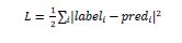
As we know that mxnet.gluon.loss.loss will calculate the MSE(Mean Squared Error) between label and prediction (pred). It is done with the help of following formula:
gluon.parameter
mxnet.gluon.parameter is a container that holds the parameters i.e. weights of the Blocks.
Methods and their parameters
Following are some of the important methods and their parameters covered by mxnet.gluon.parameter training module −
| Methods and its Parameters | Definition |
|---|---|
| cast(dtype) | This method will cast data and gradient of this Parameter to a new data type. |
| data([ctx]) | This method will return a copy of this parameter on one context. |
| grad([ctx]) | This method will return a gradient buffer for this parameter on one context. |
| initialize([init, ctx, default_init, ]) | This method will initialize parameter and gradient arrays. |
| list_ctx() | This method will return a list of contexts this parameter is initialized on. |
| list_data() | This method will return copies of this parameter on all contexts. It will be done in the same order as creation. |
| list_grad() | This method will return gradient buffers on all contexts. This will be done in the same order as values(). |
| list_row_sparse_data(row_id) | This method will return copies of the row_sparse parameter on all contexts. This will be done in the same order as creation. |
| reset_ctx(ctx) | This method will re-assign Parameter to other contexts. |
| row_sparse_data(row_id) | This method will return a copy of the row_sparse parameter on the same context as row_ids. |
| set_data(data) | This method will set this parameters value on all contexts. |
| var() | This method will return a symbol representing this parameter. |
| zero_grad() | This method will set the gradient buffer on all contexts to 0. |
Implementation Example
In the example below, we will initialize parameters and the gradients arrays by using initialize() method as follows −
weight = mx.gluon.Parameter('weight', shape=(2, 2))
weight.initialize(ctx=mx.cpu(0))
weight.data()
Output
The output is mentioned below −
[[-0.0256899 0.06511251]
[-0.00243821 -0.00123186]]
<NDArray 2x2 @cpu(0)>
Example
weight.grad()
Output
The output is given below −
[[0. 0.]
[0. 0.]]
<NDArray 2x2 @cpu(0)>
Example
weight.initialize(ctx=[mx.gpu(0), mx.gpu(1)])
weight.data(mx.gpu(0))
Output
You will see the following output −
[[-0.00873779 -0.02834515]
 [ 0.05484822 -0.06206018]]
<NDArray 2x2 @gpu(0)>
Example
weight.data(mx.gpu(1))
Output
When you execute the above code, you should see the following output −
[[-0.00873779 -0.02834515]
 [ 0.05484822 -0.06206018]]
<NDArray 2x2 @gpu(1)>
gluon.trainer
mxnet.gluon.trainer applies an Optimizer on a set of parameters. It should be used together with autograd.
Methods and their parameters
Following are some of the important methods and their parameters covered by mxnet.gluon.trainer training module −
| Methods and its Parameters | Definition |
|---|---|
| allreduce_grads() | This method will reduce the gradients from different contexts for each parameter (weight). |
| load_states(fname) | As name implies, this method will load trainer states. |
| save_states(fname) | As name implies, this method will save trainer states. |
| set_learning_rate(lr) | This method will set a new learning rate of the optimizer. |
| step(batch_size[, ignore_stale_grad]) | This method will make one step of parameter update. It should be called after autograd.backward() and outside of record() scope. |
| update(batch_size[, ignore_stale_grad]) | This method will also make one step of parameter update. It should be called after autograd.backward() and outside of record() scope and after trainer.update(). |
Data Modules
The data modules of Gluon are explained below −
gluon.data
Gluon provides a large number of build-in dataset utilities in gluon.data module. That is the reason it is called the data module.
Classes and their parameters
Following are some of the important methods and their parameters covered by mxnet.gluon.data core module. These methods are typically related to Datasets, Sampling, and DataLoader.
| Methods and its Parameters | Definition |
|---|---|
| ArrayDataset(*args) | This method represents a dataset which combines two or more than two dataset-like objects. For example, Datasets, lists, arrays, etc. |
| BatchSampler(sampler, batch_size[, last_batch]) | This method wraps over another Sampler. Once wrapped it returns the mini batches of samples. |
| DataLoader(dataset[, batch_size, shuffle, ]) | Similar to BatchSampler but this method loads data from a dataset. Once loaded it returns the mini batches of data. |
| This represents the abstract dataset class. | |
| FilterSampler(fn, dataset) | This method represents the samples elements from a Dataset for which fn (function) returns True. |
| RandomSampler(length) | This method represents samples elements from [0, length) randomly without replacement. |
| RecordFileDataset(filename) | It represents a dataset wrapping over a RecordIO file. The extension of the file is .rec. |
| Sampler | This is the base class for samplers. |
| SequentialSampler(length[, start]) | It represents the sample elements from the set [start, start+length) sequentially. |
| It represents the sample elements from the set [start, start+length) sequentially. | This represents the simple Dataset wrapper especially for lists and arrays. |
Implementation Examples
In the example below, we are going to use gluon.data.BatchSampler() API, which wraps over another sampler. It returns the mini batches of samples.
import mxnet as mx
from mxnet.gluon import data
sampler = mx.gluon.data.SequentialSampler(15)
batch_sampler = mx.gluon.data.BatchSampler(sampler, 4, 'keep')
list(batch_sampler)
Output
The output is mentioned below −
[[0, 1, 2, 3], [4, 5, 6, 7], [8, 9, 10, 11], [12, 13, 14]]
gluon.data.vision.datasets
Gluon provides a large number of pre-defined vision dataset functions in gluon.data.vision.datasets module.
Classes and their parameters
MXNet provides us useful and important datasets, whose classes and parameters are given below −
| Classes and its Parameters | Definition |
|---|---|
| MNIST([root, train, transform]) | This is a useful dataset providing us the handwritten digits. The url for MNIST dataset is http://yann.lecun.com/exdb/mnist |
| FashionMNIST([root, train, transform]) | This dataset consists of Zalandos article images consisting of fashion products. It is a drop-in replacement of original MNIST dataset. You can get this dataset from https://github.com/zalandoresearch/fashion-mnist |
| CIFAR10([root, train, transform]) | This is an image classification dataset from https://www.cs.toronto.edu/~kriz/cifar.html. In this dataset each sample is an image with shape (32, 32, 3). |
| CIFAR100([root, fine_label, train, transform]) | This is CIFAR100 image classification dataset from https://www.cs.toronto.edu/~kriz/cifar.html. It also has each sample is an image with shape (32, 32, 3). |
| ImageRecordDataset (filename[, flag, transform]) | This dataset is wrapping over a RecordIO file that contains images. In this each sample is an image with its corresponding label. |
| ImageFolderDataset (root[, flag, transform]) | This is a dataset for loading image files that are stored in a folder structure. |
| ImageListDataset ([root, imglist, flag]) | This is a dataset for loading image files that are specified by a list of entries. |
Example
In the example below, we are going to show the use of ImageListDataset(), which is used for loading image files that are specified by a list of entries −
# written to text file *.lst

0 0 root/cat/0001.jpg
1 0 root/cat/xxxa.jpg
2 0 root/cat/yyyb.jpg
3 1 root/dog/123.jpg
4 1 root/dog/023.jpg
5 1 root/dog/wwww.jpg

# A pure list, each item is a list [imagelabel: float or list of float, imgpath]

[[0, root/cat/0001.jpg]
[0, root/cat/xxxa.jpg]
[0, root/cat/yyyb.jpg]
[1, root/dog/123.jpg]
[1, root/dog/023.jpg]
[1, root/dog/wwww.jpg]]
Utility Modules
The utility modules in Gluon are as follows −
gluon.utils
Gluon provides a large number of build-in parallelisation utility optimiser in gluon.utils module. It provides variety of utilities for training. That is the reason it is called the utility module.
Functions and their parameters
Following are the functions and their parameters consisting in this utility module named gluon.utils −
| Functions and its Parameters | Definition |
|---|---|
| split_data(data, num_slice[, batch_axis, ]) | This function is usually use for data parallelism and each slice is sent to one device i.e. GPU. It splits an NDArray into num_slice slices along batch_axis. |
| split_and_load(data, ctx_list[, batch_axis, ]) | This function splits an NDArray into len(ctx_list) slices along batch_axis. The only difference from above split_data () function is that, it also loads each slice to one context in ctx_list. |
| clip_global_norm(arrays, max_norm[, ]) | The job of this function is to rescale NDArrays in such a way that the sum of their 2-norm is smaller than max_norm. |
| check_sha1(filename, sha1_hash) | This function will check whether the sha1 hash of the file content matches the expected hash or not. |
| download(url[, path, overwrite, sha1_hash, ]) | As name specifies, this function will download a given URL. |
| replace_file(src, dst) | This function will implement atomic os.replace. it will be done with Linux and OSX. |
