SymPy - Quick Guide

---

---

SymPy - Introduction

SymPy is a Python library for performing symbolic computation. It is a computer algebra system (CAS) that can be used either as a standalone application, as a library to other applications. Its live session is also available at https://live.sympy.org/. Since it is a pure Python library, it can be used as interactive mode and as a programmatic application. SymPy has now become a popular symbolic library for the scientific Python ecosystem.

SymPy has a wide range of features applicable in the field of basic symbolic arithmetic, calculus, algebra, discrete mathematics, quantum physics, etc. SymPy is capable of formatting the results in variety of formats including LaTeX, MathML, etc. SymPy is distributed under New BSD License. A team of developers led by Ondřej Čertík and Aaron Meurer published first version of SymPy in 2007. Its current version is 1.5.1.

Some of the areas of applications of SymPy are −

• Polynomials
• Calculus
• Discrete maths
• Matrices
• Geometry
• Plotting
• Physics
• Statistics
• Combinatorics

SymPy - Installation

SymPy has one important prerequisite library named mpmath. It is a Python library for real and complex floating-point arithmetic with arbitrary precision. However, Python's package installer PIP installs it automatically when SymPy is installed as follows −

pip install sympy

Other Python distributions such as Anaconda, Enthought Canopy, etc., may have SymPy already bundled in it. To verify, you can type the following in the Python prompt −

>>> import sympy
>>> sympy.__version__

And you get the below output as the current version of sympy −

'1.5.1'

Source code of SymPy package is available at https://github.com/sympy/sympy.

SymPy - Symbolic Computation

Symbolic computation refers to development of algorithms for manipulating mathematical expressions and other mathematical objects. Symbolic computation integrates mathematics with computer science to solve mathematical expressions using mathematical symbols. A Computer Algebra System (CAS) such as SymPy evaluates algebraic expressions exactly (not approximately) using the same symbols that are used in traditional manual method. For example, we calculate square root of a number using Python's math module as given below −

>>> import math 
>>> print (math.sqrt(25), math.sqrt(7))

The output for the above code snippet is as follows −

5.0 2.6457513110645907

As you can see, square root of 7 is calculated approximately. But in SymPy square roots of numbers that are not perfect squares are left unevaluated by default as given below −

>>> import sympy 
>>> print (sympy.sqrt(7))

The output for the above code snippet is as follows −

sqrt(7)

It is possible to simplify and show result of expression symbolically with the code snippet below −

>>> import math
>>> print (math.sqrt(12))

The output for the above code snippet is as follows −

3.4641016151377544

You need to use the below code snippet to execute the same using sympy −

##sympy output 
>>> print (sympy.sqrt(12))

And the output for that is as follows −

2*sqrt(3)

SymPy code, when run in Jupyter notebook, makes use of MathJax library to render mathematical symbols in LatEx form. It is shown in the below code snippet −

>>> from sympy import * 
>>> x=Symbol ('x') 
>>> expr = integrate(x**x, x) 
>>> expr

On executing the above command in python shell, following output will be generated −

Integral(x**x, x)

Which is equivalent to

$\int \mathrm{x}^{x}\,\mathrm{d}x$

The square root of a non-perfect square can be represented by Latex as follows using traditional symbol −

>>> from sympy import * 
>>> x=7 
>>> sqrt(x)

The output for the above code snippet is as follows −

$\sqrt7$

A symbolic computation system such as SymPy does all sorts of computations (such as derivatives, integrals, and limits, solve equations, work with matrices) symbolically. SymPy package has different modules that support plotting, printing (like LATEX), physics, statistics, combinatorics, number theory, geometry, logic, etc.

SymPy - Numbers

The core module in SymPy package contains Number class which represents atomic numbers. This class has two subclasses: Float and Rational class. Rational class is further extended by Integer class.

Float class represents a floating point number of arbitrary precision.

>>> from sympy import Float 
>>> Float(6.32)

The output for the above code snippet is as follows −

6.32

SymPy can convert an integer or a string to float.

>>> Float(10)

10.0

Float('1.33E5')# scientific notation

133000.0

While converting to float, it is also possible to specify number of digits for precision as given below −

>>> Float(1.33333,2)

The output for the above code snippet is as follows −

1.3

A representation of a number (p/q) is represented as object of Rational class with q being a non-zero number.

>>> Rational(3/4)

The output for the above code snippet is as follows −

$\frac{3}{4}$

If a floating point number is passed to Rational() constructor, it returns underlying value of its binary representation

>>> Rational(0.2)

The output for the above code snippet is as follows −

$\frac{3602879701896397}{18014398509481984}$

For simpler representation, specify denominator limitation.

>>> Rational(0.2).limit_denominator(100)

The output for the above code snippet is as follows −

$\frac{1}{5}$

When a string is passed to Rational() constructor, a rational number of arbitrary precision is returned.

>>> Rational("3.65")

The output for the above code snippet is as follows −

$\frac{73}{20}$

Rational object can also be obtained if two number arguments are passed. Numerator and denominator parts are available as properties.

>>> a=Rational(3,5) 
>>> print (a) 
>>> print ("numerator:{}, denominator:{}".format(a.p, a.q))

The output for the above code snippet is as follows −

3/5

numerator:3, denominator:5

>>> a

The output for the above code snippet is as follows −

$\frac{3}{5}$

Integer class in SymPy represents an integer number of any size. The constructor can accept a Float or Rational number, but the fractional part is discarded

>>> Integer(10)

The output for the above code snippet is as follows −

10

>>> Integer(3.4)

The output for the above code snippet is as follows −

3

>>> Integer(2/7)

The output for the above code snippet is as follows −

0

SymPy has a RealNumber class that acts as alias for Float. SymPy also defines Zero and One as singleton classes accessible with S.Zero and S.One respectively as shown below −

>>> S.Zero

The output is as follows −

0

>>> S.One

The output is as follows −

1

Other predefined Singleton number objects are Half, NaN, Infinity and ImaginaryUnit

>>> from sympy import S 
>>> print (S.Half)

The output is as follows −

½

>>> print (S.NaN)

The output is as follows −

nan

Infinity is available as oo symbol object or S.Infinity

>>> from sympy import oo 
>>> oo

The output for the above code snippet is as follows −

$\infty$

>>> S.Infinity

The output for the above code snippet is as follows −

$\infty$

ImaginaryUnit number can be imported as I symbol or accessed as S.ImaginaryUnit and represents square root of -1

>>> from sympy import I 
>>> I

When you execute the above code snippet, you get the following output −

i

>>> S.ImaginaryUnit

The output of the above snippet is as follows −

i

>>> from sympy import sqrt 
>>> i=sqrt(-1) 
>>> i*i

When you execute the above code snippet, you get the following output −

-1

SymPy - Symbols

Symbol is the most important class in symPy library. As mentioned earlier, symbolic computations are done with symbols. SymPy variables are objects of Symbols class.

Symbol() function's argument is a string containing symbol which can be assigned to a variable.

>>> from sympy import Symbol 
>>> x=Symbol('x') 
>>> y=Symbol('y') 
>>> expr=x**2+y**2 
>>> expr

The above code snippet gives an output equivalent to the below expression −

$x^2 + y^2$

A symbol may be of more than one alphabets.

>>> s=Symbol('side') 
>>> s**3

The above code snippet gives an output equivalent to the below expression −

$side^3$

SymPy also has a Symbols() function that can define multiple symbols at once. String contains names of variables separated by comma or space.

>>> from sympy import symbols 
>>> x,y,z=symbols("x,y,z")

In SymPy's abc module, all Latin and Greek alphabets are defined as symbols. Hence, instead of instantiating Symbol object, this method is convenient.

>>> from sympy.abc import x,y,z

However, the names C, O, S, I, N, E and Q are predefined symbols. Also, symbols with more than one alphabets are not defined in abc module, for which you should use Symbol object as above. The abc module defines special names that can detect definitions in default SymPy namespace. clash1 contains single letters and clash2 has multi letter clashing symbols

>>> from sympy.abc import _clash1, _clash2 
>>> _clash1

The output of the above snippet is as follows −

{'C': C, 'O': O, 'Q': Q, 'N': N, 'I': I, 'E': E, 'S': S}

>>> _clash2

The output of the above snippet is as follows −

{'beta': beta, 'zeta': zeta, 'gamma': gamma, 'pi': pi}

Indexed symbols can be defined using syntax similar to range() function. Ranges are indicated by a colon. Type of range is determined by the character to the right of the colon. If itr is a digit, all contiguous digits to the left are taken as the nonnegative starting value. All contiguous digits to the right are taken as 1 greater than the ending value.

>>> from sympy import symbols 
>>> symbols('a:5')

The output of the above snippet is as follows −

(a0, a1, a2, a3, a4)

>>> symbols('mark(1:4)')

The output of the above snippet is as follows −

(mark1, mark2, mark3)

SymPy - Substitution

One of the most basic operations to be performed on a mathematical expression is substitution. The subs() function in SymPy replaces all occurrences of first parameter with second.

>>> from sympy.abc import x,a 
>>> expr=sin(x)*sin(x)+cos(x)*cos(x) 
>>> expr

The above code snippet gives an output equivalent to the below expression −

$\sin^2(x)+\cos^2(x)$

>>> expr.subs(x,a)

The above code snippet gives an output equivalent to the below expression −

$\sin^2(a)+\cos^2(a)$

This function is useful if we want to evaluate a certain expression. For example, we want to calculate values of following expression by substituting a with 5.

>>> expr=a*a+2*a+5 
>>> expr

The above code snippet gives an output equivalent to the below expression −

$a^2 + 2a + 5$

expr.subs(a,5)

The above code snippet gives the following output −

40

>>> from sympy.abc import x 
>>> from sympy import sin, pi 
>>> expr=sin(x) 
>>> expr1=expr.subs(x,pi) 
>>> expr1

The above code snippet gives the following output −

0

This function is also used to replace a subexpression with another subexpression. In following example, b is replaced by a+b.

>>> from sympy.abc import a,b 
>>> expr=(a+b)**2 
>>> expr1=expr.subs(b,a+b) 
>>> expr1

The above code snippet gives an output equivalent to the below expression −

$(2a + b)^2$

SymPy - sympify() function

The sympify() function is used to convert any arbitrary expression such that it can be used as a SymPy expression. Normal Python objects such as integer objects are converted in SymPy. Integer, etc.., strings are also converted to SymPy expressions.

>>> expr="x**2+3*x+2" 
>>> expr1=sympify(expr) 
>>> expr1 
>>> expr1.subs(x,2)

The above code snippet gives the following output −

12

Any Python object can be converted in SymPy object. However, since the conversion internally uses eval() function, unsanitized expression should not be used, else SympifyError is raised.

>>> sympify("x***2")
---------------------------------------------------------------------------

SympifyError: Sympify of expression 'could not parse 'x***2'' failed, because of exception being raised.

The sympify() function takes following arguments: * strict: default is False. If set to True, only the types for which an explicit conversion has been defined are converted. Otherwise, SympifyError is raised. * evaluate: If set to False, arithmetic and operators will be converted into their SymPy equivalents without evaluating expression.

>>> sympify("10/5+4/2")

The above code snippet gives the following output −

4

>>> sympify("10/5+4/2", evaluate=False)

The above code snippet gives the following output −

$\frac{10}{5}+\frac{4}{2}$

SymPy - evalf() function

This function evaluates a given numerical expression upto a given floating point precision upto 100 digits. The function also takes subs parameter a dictionary object of numerical values for symbols. Consider following expression

>>> from sympy.abc import r 
>>> expr=pi*r**2 
>>> expr

The above code snippet gives an output equivalent to the below expression −

$\Pi{r^2}$

To evaluate above expression using evalf() function by substituting r with 5

>>> expr.evalf(subs={r:5})

The above code snippet gives the following output −

78.5398163397448

By default, floating point precision is upto 15 digits which can be overridden by any number upto 100. Following expression is evaluated upto 20 digits of precision.

>>> expr=a/b 
>>> expr.evalf(20, subs={a:100, b:3})

The above code snippet gives the following output −

33.333333333333333333

SymPy - Lambdify() function

The lambdify function translates SymPy expressions into Python functions. If an expression is to be evaluated over a large range of values, the evalf() function is not efficient. lambdify acts like a lambda function, except it converts the SymPy names to the names of the given numerical library, usually NumPy. By default, lambdify on implementations in the math standard library.

>>> expr=1/sin(x) 
>>> f=lambdify(x, expr) 
>>> f(3.14)

The above code snippet gives the following output −

627.8831939138764

The expression might have more than one variables. In that case, first argument to lambdify() function is a list of variables, followed by the expression to be evaluated.

>>> expr=a**2+b**2 
>>> f=lambdify([a,b],expr) 
>>> f(2,3)

The above code snippet gives the following output −

13

However, to leverage numpy library as numerical backend, we have to define the same as an argument for lambdify() function.

>>> f=lambdify([a,b],expr, "numpy")

We use two numpy arrays for two arguments a and b in the above function. The execution time is considerably fast in case of numpy arrays.

>>> import numpy 
>>> l1=numpy.arange(1,6) 
>>> l2=numpy.arange(6,11) 
>>> f(l1,l2)

The above code snippet gives the following output −

array([ 37, 53, 73, 97, 125], dtype=int32)

SymPy - Logical Expressions

Boolean functions are defined in sympy.basic.booleanarg module. It is possible to build Boolean expressions with the standard python operators & (And), | (Or), ~ (Not) as well as with >> and <<. Boolean expressions inherit from Basic class defined in SymPy's core module.

BooleanTrue function

This function is equivalent of True as in core Python. It returns a singleton that can be retrieved by S.true.

>>> from sympy import * 
>>> x=sympify(true) 
>>> x, S.true

The above code snippet gives the following output −

(True, True)

BooleanFalse function

Similarly, this function is equivalent to Boolean False in Python and can be accessed by S.false

>>> from sympy import * 
>>> x=sympify(false) 
>>> x, S.false

The above code snippet gives the following output −

(False, False)

And function

A logical AND function evaluates its two arguments and returns False if either of them is False. The function emulates & operator.

>>> from sympy import * 
>>> from sympy.logic.boolalg import And 
>>> x,y=symbols('x y') 
>>> x=True 
>>> y=True 
>>> And(x,y), x"&"y

The above code snippet gives the following output −

(True, True)

>>> y=False 
>>> And(x,y), x"&"y

The above code snippet gives the following output −

(False, False)

Or function

This function evaluates two Boolean arguments and returns True if either of them is True. The | operator conveniently emulates its behaviour.

>>> from sympy import * 
>>> from sympy.logic.boolalg import Or 
>>> x,y=symbols('x y') 
>>> x=True 
>>> y=False 
>>> Or(x,y), x|y

The above code snippet gives the following output −

(True, True)

>>> x=False 
>>> y=False 
>>> Or(x,y), x|y

The above code snippet gives the following output −

(False, False)

Not Function

A Logical Not function results in negation of the Boolean argument. It returns True if its argument is False and returns False if True. The ~ operator performs the operation similar to Not function. It is shown in the example below −

>>> from sympy import * 
>>> from sympy.logic.boolalg import Or, And, Not 
>>> x,y=symbols('x y') 
>>> x=True 
>>> y=False 
>>> Not(x), Not(y)

The above code snippet gives the following output −

(False, True)

>>> Not(And(x,y)), Not(Or(x,y))

The above code snippet gives the following output −

(True, False)

Xor Function

The Logical XOR (exclusive OR) function returns True if an odd number of the arguments are True and the rest are False and returns False if an even number of the arguments are True and the rest are False. Similar operation is performed by ^ operator.

>>> from sympy import * 
>>> from sympy.logic.boolalg import Xor 
>>> x,y=symbols('x y') 
>>> x=True 
>>> y=False

>>> Xor(x,y), x^y

The above code snippet gives the following output −

(True, True)

>>> a,b,c,d,e=symbols('a b c d e') 
>>> a,b,c,d,e=(True, False, True, True, False) 
>>> Xor(a,b,c,d,e)

The above code snippet gives the following output −

True

In above case, three (odd number) arguments are True, hence Xor returns true. However, if number of True arguments is even, it results in False, as shown below −

>>> a,b,c,d,e=(True, False, False, True, False) 
>>> Xor(a,b,c,d,e)

The above code snippet gives the following output −

False

Nand Function

This function performs Logical NAND operation. It evaluates its arguments and returns True if any of them are False, and False if they are all True.

>>> from sympy import * 
>>> from sympy.logic.boolalg import Nand 
>>> a,b,c=symbols('a b c') 
>>> a,b,c=(True, False, True) 
>>> Nand(a,b,c), Nand(a,c)

The above code snippet gives the following output −

(True, False)

Nor Function

This function performs Logical NOR operation. It evaluates its arguments and returns False if any of them are True, and True if they are all False.

>>> from sympy import * 
>>> from sympy.logic.boolalg import Nor 
>>> a,b,c=symbols('a b c') 
>>> a,b,c=(True, False, True) 
>>> Nor(a,b,c), Nor(a,c)

The above code snippet gives the following output −

(False, False)

Note that even though SymPy provides ^ operator for Xor, ~ for Not, | for Or and & for And functions as convenience, their normal use in Python is as bitwise operators. Hence, if operands are integers, results would be different.

Equivalent function

This function returns equivalence relation. Equivalent(A, B) is True if and only if A and B are both True or both False. The function returns True if all of the arguments are logically equivalent. Returns False otherwise.

>>> from sympy import * 
>>> from sympy.logic.boolalg import Equivalent 
>>> a,b,c=symbols('a b c') 
>>> a,b,c=(True, False, True) 
>>> Equivalent(a,b), Equivalent(a,c)

The above code snippet gives the following output −

(False, True)

ITE function

This function acts as If then else clause in a programming language.ITE(A, B, C) evaluates and returns the result of B if A is true else it returns the result of C. All args must be Booleans.

>>> from sympy import * >>> from sympy.logic.boolalg import ITE >>> a,b,c=symbols('a b c') >>> a,b,c=(True, False, True) 
>>> ITE(a,b,c), ITE(a,c,b)

The above code snippet gives the following output −

(False, True)

SymPy - Querying

The assumptions module in SymPy package contains tools for extracting information about expressions. The module defines ask() function for this purpose.

sympy.assumptions.ask(property)

Following properties provide useful information about an expression −

algebraic(x)

To be algebraic, a number must be a root of a non-zero polynomial equation with rational coefficients. √2 because √2 is a solution to x2 − 2 = 0, so it is algebraic.

complex(x)

Complex number predicate. It is true if and only if x belongs to the set of complex numbers.

composite(x)

Composite number predicate returned by ask(Q.composite(x)) is true if and only if x is a positive integer and has at least one positive divisor other than 1 and the number itself.

even, odd

The ask() returns true of x is in the set of even numbers and set of odd numbers respectively.

imaginary

This property represents Imaginary number predicate. It is true if x can be written as a real number multiplied by the imaginary unit I.

integer

This property returned by Q.integer(x) returns true of x belong to set of even numbers.

rational, irrational

Q.irrational(x) is true if and only if x is any real number that cannot be expressed as a ratio of integers. For example, pi is an irrational number.

positive, negative

Predicates to check if number is positive or negative

zero, nonzero

Predicates to heck if a number is zero or not

>>> from sympy import * 
>>> x=Symbol('x') 
>>> x=10 
>>> ask(Q.algebraic(pi))
False
>>> ask(Q.complex(5-4*I)), ask( Q.complex(100))
(True, True)
>>> x,y=symbols("x y") 
>>> x,y=5,10 
>>> ask(Q.composite(x)), ask(Q.composite(y))
(False, True)
>>> ask(Q.even(x)), ask(Q.even(y))
(False, True)
>>> x,y= 2*I, 4+5*I 
>>> ask(Q.imaginary(x)), ask(Q.imaginary(y))
(True, False)
>>> x,y=5,10 
>>> ask(Q.even(x)), ask(Q.even(y)), ask(Q.odd(x)), ask(Q.odd(y))
(False, True, True, False)
>>> x,y=5,-5 
>>> ask(Q.positive(x)), ask(Q.negative(y)), ask(Q.positive(x)), ask(Q.negative(y))
(True, True, True, True)
>>> ask(Q.rational(pi)), ask(Q.irrational(S(2)/3))
(False, False)
>>> ask(Q.zero(oo)), ask(Q.nonzero(I))
(False, False)

SymPy - Simplification

Sympy has powerful ability to simplify mathematical expressions. There are many functions in SymPy to perform various kinds of simplification. A general function called simplify() is there that attempts to arrive at the simplest form of an expression.

simplify

This function is defined in sympy.simplify module. simplify() tries to apply intelligent heuristics to make the input expression “simpler”. Following code shows simplifies expression $sin^2(x)+cos^2(x)$.

>>> from sympy import * 
>>> x=Symbol('x')
>>> expr=sin(x)**2 + cos(x)**2 
>>> simplify(expr)

The above code snippet gives the following output −

1

expand

The expand() is one of the most common simplification functions in SymPy, used in expanding polynomial expressions. For example −

>>> a,b=symbols('a b') 
>>> expand((a+b)**2)

The above code snippet gives an output equivalent to the below expression −

$a^2 + 2ab + b^2$

>>> expand((a+b)*(a-b))

The above code snippet gives an output equivalent to the below expression −

$a^2 - b^2$

The expand() function makes expressions bigger, not smaller. Usually this is the case, but often an expression will become smaller upon calling expand() on it.

>>> expand((x + 1)*(x - 2) - (x - 1)*x)

The above code snippet gives the following output −

-2

factor

This function takes a polynomial and factors it into irreducible factors over the rational numbers.

>>> x,y,z=symbols('x y z') 
>>> expr=(x**2*z + 4*x*y*z + 4*y**2*z) 
>>> factor(expr)

The above code snippet gives an output equivalent to the below expression −

$z(x + 2y)^2$

>>> factor(x**2+2*x+1)

The above code snippet gives an output equivalent to the below expression −

$(x + 1)^2$

The factor() function is the opposite of expand(). Each of the factors returned by factor() is guaranteed to be irreducible. The factor_list() function returns a more structured output.

>>> expr=(x**2*z + 4*x*y*z + 4*y**2*z) 
>>> factor_list(expr)

The above code snippet gives an output equivalent to the below expression −

(1, [(z, 1), (x + 2*y, 2)])

collect

This function collects additve terms of an expression with respect to a list of expression up to powers with rational exponents.

>>> expr=x*y + x - 3 + 2*x**2 - z*x**2 + x**3 
>>> expr

The above code snippet gives an output equivalent to the below expression −

$x^3 + x^2z + 2x^2 + xy + x - 3$

The collect() function on this expression results as follows −

>>> collect(expr,x)

The above code snippet gives an output equivalent to the below expression −

$x^3 + x^2(2 - z) + x(y + 1) - 3$

>>> expr=y**2*x + 4*x*y*z + 4*y**2*z+y**3+2*x*y 
>>> collect(expr,y)

The above code snippet gives an output equivalent to the below expression −

$Y^3+Y^2(x+4z)+y(4xz+2x)$

cancel

The cancel() function will take any rational function and put it into the standard canonical form, p/q, where p and q are expanded polynomials with no common factors. The leading coefficients of p and q do not have denominators i.e., they are integers.

>>> expr1=x**2+2*x+1 
>>> expr2=x+1 
>>> cancel(expr1/expr2)

The above code snippet gives an output equivalent to the below expression −

$x+1$

>>> expr = 1/x + (3*x/2 - 2)/(x - 4) 
>>> expr

The above code snippet gives an output equivalent to the below expression −

$\frac{\frac{3x}{2} - 2}{x - 4} + \frac{1}{x}$

>>> cancel(expr)

The above code snippet gives an output equivalent to the below expression −

$\frac{3x^2 - 2x - 8}{2x^2 - 8}$

>>> expr=1/sin(x)**2 
>>> expr1=sin(x) 
>>> cancel(expr1*expr)

The above code snippet gives an output equivalent to the below expression −

$\frac{1}{\sin(x)}$

trigsimp

This function is used to simplify trigonometric identities. It may be noted that naming conventions for inverse trigonometric functions is to append an a to the front of the function’s name. For example, the inverse cosine, or arc cosine, is called acos().

>>> from sympy import trigsimp, sin, cos 
>>> from sympy.abc import x, y
>>> expr = 2*sin(x)**2 + 2*cos(x)**2 
>>> trigsimp(expr)

2

The trigsimp function uses heuristics to apply the best suitable trigonometric identity.

powersimp

This function reduces given expression by combining powers with similar bases and exponents.

>>> expr=x**y*x**z*y**z 
>>> expr

The above code snippet gives an output equivalent to the below expression −

$x^y x^z y^z$

>>> powsimp(expr)

The above code snippet gives an output equivalent to the below expression −

$x^{y+z} y^z$

You can make powsimp() only combine bases or only combine exponents by changing combine=’base’ or combine=’exp’. By default, combine=’all’, which does both.If force is True then bases will be combined without checking for assumptions.

>>> powsimp(expr, combine='base', force=True)

The above code snippet gives an output equivalent to the below expression −

$x^y(xy)^z$

combsimp

Combinatorial expressions involving factorial an binomials can be simplified by using combsimp() function. SymPy provides a factorial() function

>>> expr=factorial(x)/factorial(x - 3) 
>>> expr

The above code snippet gives an output equivalent to the below expression −

$\frac{x!}{(x - 3)!}$

To simplify above combinatorial expression we use combsimp() function as follows −

>>> combsimp(expr)

The above code snippet gives an output equivalent to the below expression −

$x(x-2)(x-1)$

The binomial(x, y) is the number of ways to choose y items from a set of x distinct items. It is also often written as xCy.

>>> binomial(x,y)

The above code snippet gives an output equivalent to the below expression −

$(\frac{x}{y})$

>>> combsimp(binomial(x+1, y+1)/binomial(x, y))

The above code snippet gives an output equivalent to the below expression −

$\frac{x + 1}{y + 1}$

logcombine

This function takes logarithms and combines them using the following rules −

• log(x) + log(y) == log(x*y) if both are positive
• a*log(x) == log(x**a) if x is positive and a is real

>>> logcombine(a*log(x) + log(y) - log(z))

The above code snippet gives an output equivalent to the below expression −

$a\log(x) + \log(y) - \log(z)$

If force parameter of this function is set to True then the assumptions above will be assumed to hold if there is no assumption already in place on a quantity.

>>> logcombine(a*log(x) + log(y) - log(z), force=True)

The above code snippet gives an output equivalent to the below expression −

$\log\frac{x^a y}{z}$

SymPy - Derivative

The derivative of a function is its instantaneous rate of change with respect to one of its variables. This is equivalent to finding the slope of the tangent line to the function at a point.we can find the differentiation of mathematical expressions in the form of variables by using diff() function in SymPy package.

diff(expr, variable)
>>> from sympy import diff, sin, exp 
>>> from sympy.abc import x,y 
>>> expr=x*sin(x*x)+1 >>> expr

The above code snippet gives an output equivalent to the below expression −

$x\sin(x^2) + 1$

>>> diff(expr,x)

The above code snippet gives an output equivalent to the below expression −

$2x^2\cos(x^2) + \sin(x^2)$

>>> diff(exp(x**2),x)

The above code snippet gives an output equivalent to the below expression −

2xe^x2

To take multiple derivatives, pass the variable as many times as you wish to differentiate, or pass a number after the variable.

>>> diff(x**4,x,3)

The above code snippet gives an output equivalent to the below expression −

$24x$

>>> for i in range(1,4): print (diff(x**4,x,i))

The above code snippet gives the below expression −

4*x**3

12*x**2

24*x

It is also possible to call diff() method of an expression. It works similarly as diff() function.

>>> expr=x*sin(x*x)+1 
>>> expr.diff(x)

The above code snippet gives an output equivalent to the below expression −

$2x^2\cos(x^2) + \sin(x^2)$

An unevaluated derivative is created by using the Derivative class. It has the same syntax as diff() function. To evaluate an unevaluated derivative, use the doit method.

>>> from sympy import Derivative 
>>> d=Derivative(expr) 
>>> d

The above code snippet gives an output equivalent to the below expression −

$\frac{d}{dx}(x\sin(x^2)+1)$

>>> d.doit()

The above code snippet gives an output equivalent to the below expression −

$2x^2\cos(x^2) + \sin(x^2)$

SymPy - Integration

The SymPy package contains integrals module. It implements methods to calculate definite and indefinite integrals of expressions. The integrate() method is used to compute both definite and indefinite integrals. To compute an indefinite or primitive integral, just pass the variable after the expression.

For example −

integrate(f, x)

To compute a definite integral, pass the argument as follows −

(integration_variable, lower_limit, upper_limit)

>>> from sympy import * 
>>> x,y = symbols('x y') 
>>> expr=x**2 + x + 1 
>>> integrate(expr, x)

The above code snippet gives an output equivalent to the below expression −

$\frac{x^3}{3} + \frac{x^2}{2} + x$

>>> expr=sin(x)*tan(x) 
>>> expr 
>>> integrate(expr,x)

The above code snippet gives an output equivalent to the below expression −

$-\frac{\log(\sin(x) - 1)}{2} + \frac{\log(\sin(x) + 1)}{2} - \sin(x)$

The example of definite integral is given below −

>>> expr=exp(-x**2) 
>>> integrate(expr,(x,0,oo) )

The above code snippet gives an output equivalent to the below expression −

$\frac{\sqrt\pi}{2}$

You can pass multiple limit tuples to perform a multiple integral. An example is given below −

>>> expr=exp(-x**2 - y**2)
>>> integrate(expr,(x,0,oo),(y,0,oo))

The above code snippet gives an output equivalent to the below expression −

$\frac{\pi}{4}$

You can create unevaluated integral using Integral object, which can be evaluated by calling doit() method.

>>> expr = Integral(log(x)**2, x) 
>>> expr

The above code snippet gives an output equivalent to the below expression −

$\int \mathrm\log(x)^2 \mathrm{d}x$

>>> expr.doit()

The above code snippet gives an output equivalent to the below expression −

$x\log(x)^2 - 2xlog(x) + 2x$

Integral Transforms

SymPy supports various types of integral transforms as follows −

• laplace_transform
• fourier_transform
• sine_transform
• cosine_transform
• hankel_transform

These functions are defined in sympy.integrals.transforms module. Following examples compute Fourier transform and Laplace transform respectively.

Example 1

>>> from sympy import fourier_transform, exp 
>>> from sympy.abc import x, k 
>>> expr=exp(-x**2) 
>>> fourier_transform(expr, x, k)

On executing the above command in python shell, following output will be generated −

sqrt(pi)*exp(-pi**2*k**2)

Which is equivalent to −

$\sqrt\pi * e^{\pi^2k^2}$

Example 2

>>> from sympy.integrals import laplace_transform 
>>> from sympy.abc import t, s, a 
>>> laplace_transform(t**a, t, s)

On executing the above command in python shell, following output will be generated −

(s**(-a)*gamma(a + 1)/s, 0, re(a) > -1)

SymPy - Matrices

In Mathematics, a matrix is a two dimensional array of numbers, symbols or expressions. Theory of matrix manipulation deals with performing arithmetic operations on matrix objects, subject to certain rules.

Linear transformation is one of the important applications of matrices. Many scientific fields, specially related to Physics use matrix related applications.

SymPy package has matrices module that deals with matrix handling. It includes Matrix class whose object represents a matrix.

Note: If you want to execute all the snippets in this chapter individually, you need to import the matrix module as shown below −

>>> from sympy.matrices import Matrix

Example

>>> from sympy.matrices import Matrix 
>>> m=Matrix([[1,2,3],[2,3,1]]) 
>>> m
$\displaystyle \left[\begin{matrix}1 & 2 & 3\\2 & 3 & 1\end{matrix}\right]$

On executing the above command in python shell, following output will be generated −

[1 2 3 2 3 1]

Matrix is created from appropriately sized List objects. You can also obtain a matrix by distributing list items in specified number of rows and columns.

>>> M=Matrix(2,3,[10,40,30,2,6,9]) 
>>> M
$\displaystyle \left[\begin{matrix}10 & 40 & 30\\2 & 6 & 9\end{matrix}\right]$

On executing the above command in python shell, following output will be generated −

[10 40 30 2 6 9]

Matrix is a mutable object. The matrices module also provides ImmutableMatrix class for obtaining immutable matrix.

Basic manipulation

The shape property of Matrix object returns its size.

>>> M.shape

The output for the above code is as follows −

(2,3)

The row() and col() method respectively returns row or column of specified number.

>>> M.row(0)
$\displaystyle \left[\begin{matrix}10 & 40 & 30\end{matrix}\right]$

The output for the above code is as follows −

[10 40 30]

>>> M.col(1)
$\displaystyle \left[\begin{matrix}40\\6\end{matrix}\right]$

The output for the above code is as follows −

[40 6]

Use Python's slice operator to fetch one or more items belonging to row or column.

>>> M.row(1)[1:3]
[6, 9]

Matrix class has row_del() and col_del() methods that deletes specified row/column from given matrix −

>>> M=Matrix(2,3,[10,40,30,2,6,9]) 
>>> M.col_del(1) 
>>> M

On executing the above command in python shell, following output will be generated −

Matrix([[10, 30],[ 2, 9]])

You can apply style to the output using the following command −

$\displaystyle \left[\begin{matrix}10 & 30\\2 & 9\end{matrix}\right]$

You get the following output after executing the above code snippet −

[10 30 2 9]

>>> M.row_del(0) 
>>> M

$\displaystyle \left[\begin{matrix}2 & 9\end{matrix}\right]$

You get the following output after executing the above code snippet −

[2 9]

Similarly, row_insert() and col_insert() methods add rows or columns at specified row or column index

>>> M1=Matrix([[10,30]]) 
>>> M=M.row_insert(0,M1)
>>> M

$\displaystyle \left[\begin{matrix}10 & 30\\2 & 9\end{matrix}\right]$

You get the following output after executing the above code snippet −

[10 40 30 2 9]

>>> M2=Matrix([40,6]) 
>>> M=M.col_insert(1,M2) 
>>> M

$\displaystyle \left[\begin{matrix}10 & 40 & 30\\2 & 6 & 9\end{matrix}\right]$

You get the following output after executing the above code snippet −

[10 40 30 6 9]

Arithmetic Operations

Usual operators +, - and * are defined for performing addition, subtraction and multiplication.

>>> M1=Matrix([[1,2,3],[3,2,1]]) 
>>> M2=Matrix([[4,5,6],[6,5,4]]) 
>>> M1+M2

$\displaystyle \left[\begin{matrix}5 & 7 & 9\\9 & 7 & 5\end{matrix}\right]$

You get the following output after executing the above code snippet −

[5 7 9 9 7 5]

>>> M1-M2
$\displaystyle \left[\begin{matrix}-3 & -3 & -3\\-3 & -3 & -3\end{matrix}\right]$

You get the following output after executing the above code snippet −

[- 3 -3 -3 -3 -3 -3]

Matrix multiplication is possible only if - The number of columns of the 1st matrix must equal the number of rows of the 2nd matrix. - And the result will have the same number of rows as the 1st matrix, and the same number of columns as the 2nd matrix.

>>> M1=Matrix([[1,2,3],[3,2,1]]) 
>>> M2=Matrix([[4,5],[6,6],[5,4]]) 
>>> M1*M2
$\displaystyle \left[\begin{matrix}31 & 29\\29 & 31\end{matrix}\right]$

The output for the above code is as follows −

[31 29 29 31]

>>> M1.T
$\displaystyle \left[\begin{matrix}1 & 3\\2 & 2\\3 & 1\end{matrix}\right]$

The following output is obtained after executing the code −

[1 3 2 2 3 1]

To calculate a determinant of matrix, use det() method. A determinant is a scalar value that can be computed from the elements of a square matrix.0

>>> M=Matrix(3,3,[10,20,30,5,8,12,9,6,15])
>>> M
$\displaystyle \left[\begin{matrix}10 & 20 & 30\\5 & 8 & 12\\9 & 6 & 15\end{matrix}\right]$

The output for the above code is as follows −

[10 20 30 5 8 12 9 6 15]

>>> M.det()

The output for the above code is as follows −

-120

Matrix Constructors

SymPy provides many special type of matrix classes. For example, Identity matrix, matrix of all zeroes and ones, etc. These classes are named as eye, zeros and ones respectively. Identity matrix is a square matrix with elements falling on diagonal are set to 1, rest of the elements are 0.

Example

from sympy.matrices import eye eye(3)

Output

Matrix([[1, 0, 0], [0, 1, 0], [0, 0, 1]])

$\displaystyle \left[\begin{matrix}1 & 0 & 0\\0 & 1 & 0\\0 & 0 & 1\end{matrix}\right]$

The output for the above code is as follows −

[1 0 0 0 1 0 0 0 1]

In diag matrix, elements on diagonal are initialized as per arguments provided.

>>> from sympy.matrices import diag 
>>> diag(1,2,3)

$\displaystyle \left[\begin{matrix}1 & 0 & 0\\0 & 2 & 0\\0 & 0 & 3\end{matrix}\right]$

The output for the above code is as follows −

[1 0 0 0 2 0 0 0 3]

All elements in zeros matrix are initialized to 0.

>>> from sympy.matrices import zeros 
>>> zeros(2,3)

$\displaystyle \left[\begin{matrix}0 & 0 & 0\\0 & 0 & 0\end{matrix}\right]$

The output for the above code is as follows −

[0 0 0 0 0 0]

Similarly, ones is matrix with all elements set to 1.

>>> from sympy.matrices import ones
>>> ones(2,3)

$\displaystyle \left[\begin{matrix}1 & 1 & 1\\1 & 1 & 1\end{matrix}\right]$

The output for the above code is as follows −

[1 1 1 1 1 1]

SymPy - Function class

Sympy package has Function class, which is defined in sympy.core.function module. It is a base class for all applied mathematical functions, as also a constructor for undefined function classes.

Following categories of functions are inherited from Function class −

• Functions for complex number
• Trigonometric functions
• Functions for integer number
• Combinatorial functions
• Other miscellaneous functions

Functions for complex number

This set of functions is defined in sympy.functions.elementary.complexes module.

re

This function returns real part of an expression −

>>> from sympy import * 
>>> re(5+3*I)

The output for the above code snippet is given below −

5

>>> re(I)

The output for the above code snippet is −

0

Im

This function returns imaginary part of an expression −

>>> im(5+3*I)

The output for the above code snippet is given below −

3

>>> im(I)

The output for the above code snippet is given below −

1

sign

This function returns the complex sign of an expression.

For real expression, the sign will be −

• 1 if expression is positive
• 0 if expression is equal to zero
• -1 if expression is negative

If expression is imaginary the sign returned is −

• I if im(expression) is positive
• -I if im(expression) is negative

>>> sign(1.55), sign(-1), sign(S.Zero)

The output for the above code snippet is given below −

(1, -1, 0)

>>> sign (-3*I), sign(I*2)

The output for the above code snippet is given below −

(-I, I)

Abs

This function return absolute value of a complex number. It is defined as the distance between the origin (0,0) and the point (a,b) in the complex plane. This function is an extension of the built-in function abs() to accept symbolic values.

>>> Abs(2+3*I)

The output for the above code snippet is given below −

$\sqrt13$

conjugate

This function returns conjugate of a complex number. To find the complex conjugate we change the sign of the imaginary part.

>>> conjugate(4+7*I)

You get the following output after executing the above code snippet −

4 - 7i

Trigonometric functions

SymPy has defintions for all trigonometric ratios - sin cos, tan etc as well as well as its inverse counterparts such as asin, acos, atan etc. These functions compute respective value for given angle expressed in radians.

>>> sin(pi/2), cos(pi/4), tan(pi/6)

The output for the above code snippet is given below −

(1, sqrt(2)/2, sqrt(3)/3)

>>> asin(1), acos(sqrt(2)/2), atan(sqrt(3)/3)

The output for the above code snippet is given below −

(pi/2, pi/4, pi/6)

Functions on Integer Number

This is a set of functions to perform various operations on integer number.

ceiling

This is a univariate function which returns the smallest integer value not less than its argument. In case of complex numbers, ceiling of the real and imaginary parts separately.

>>> ceiling(pi), ceiling(Rational(20,3)), ceiling(2.6+3.3*I)

The output for the above code snippet is given below −

(4, 7, 3 + 4*I)

floor

This function returns the largest integer value not greater than its argument. In case of complex numbers, this function too takes the floor of the real and imaginary parts separately.

>>> floor(pi), floor(Rational(100,6)), floor(6.3-5.9*I)

The output for the above code snippet is given below −

(3, 16, 6 - 6*I)

frac

This function represents the fractional part of x.

>>> frac(3.99), frac(Rational(10,3)), frac(10)

The output for the above code snippet is given below −

(0.990000000000000, 1/3, 0)

Combinatorial functions

Combinatorics is a field of mathematics concerned with problems of selection, arrangement, and operation within a finite or discrete system.

factorial

The factorial is very important in combinatorics where it gives the number of ways in which n objects can be permuted. It is symbolically represented as 𝑥! This function is implementation of factorial function over nonnegative integers, factorial of a negative integer is complex infinity.

>>> x=Symbol('x') 
>>> factorial(x)

The output for the above code snippet is given below −

x!

>>> factorial(5)

The output for the above code snippet is given below −

120

>>> factorial(-1)

The output for the above code snippet is given below −

$\infty\backsim$

binomial

This function the number of ways we can choose k elements from a set of n elements.

>>> x,y=symbols('x y') 
>>> binomial(x,y)

The output for the above code snippet is given below −

$(\frac{x}{y})$

>>> binomial(4,2)

The output for the above code snippet is given below −

6

Rows of Pascal's triangle can be generated with the binomial function.

>>> for i in range(5): print ([binomial(i,j) for j in range(i+1)])

You get the following output after executing the above code snippet −

[1]

[1, 1]

[1, 2, 1]

[1, 3, 3, 1]

[1, 4, 6, 4, 1]

fibonacci

The Fibonacci numbers are the integer sequence defined by the initial terms F0=0, F1=1 and the two-term recurrence relation Fn=Fn−1+Fn−2.

>>> [fibonacci(x) for x in range(10)]

The following output is obtained after executing the above code snippet −

[0, 1, 1, 2, 3, 5, 8, 13, 21, 34]

tribonacci

The Tribonacci numbers are the integer sequence defined by the initial terms F0=0, F1=1, F2=1 and the three-term recurrence relation Fn=Fn-1+Fn-2+Fn-3.

>>> tribonacci(5, Symbol('x'))

The above code snippet gives an output equivalent to the below expression −

$x^8 + 3x^5 + 3x^2$

>>> [tribonacci(x) for x in range(10)]

The following output is obtained after executing the above code snippet −

[0, 1, 1, 2, 4, 7, 13, 24, 44, 81]

Miscellaneous Functions

Following is a list of some frequently used functions −

Min − Returns minimum value of the list. It is named Min to avoid conflicts with the built-in function min.

Max − Returns maximum value of the list. It is named Max to avoid conflicts with the built-in function max.

root − Returns nth root of x.

sqrt − Returns the principal square root of x.

cbrt − This function computes the principal cube root of x, (shortcut for x++Rational(1,3)).

The following are the examples of the above miscellaneous functions and their respective outputs −

>>> Min(pi,E)

e

>>> Max(5, Rational(11,2))

$\frac{11}{2}$

>>> root(7,Rational(1,2))

49

>>> sqrt(2)

$\sqrt2$

>>> cbrt(1000)

10

SymPy - Quaternion

In mathematics, Quaternion number system is an extension of complex numbers. Each Quaternion object contains four scalar variables and four dimensions, one real dimension and three imaginary dimensions.

Quaternion is represented by following expression −

q=a+bi+cj+dk

where a, b, c and d are real numbers and i, j, k are quaternion units such that,i2==j2==k2==ijk

The sympy.algebras.quaternion module has Quaternion class.

>>> from sympy.algebras.quaternion import Quaternion 
>>> q=Quaternion(2,3,1,4) 
>>> q

The above code snippet gives an output equivalent to the below expression −

$2 + 3i + 1j + 4k$

Quaternions are used in pure mathematics, as well as in applied mathematics, computer graphics, computer vision, etc.

>>> from sympy import * 
>>> x=Symbol('x') 
>>> q1=Quaternion(x**2, x**3, x) >>> q1

The above code snippet gives an output equivalent to the below expression −

$x^2 + x^3i + xj + 0k$

Quaternion object can also have imaginary co-efficients

>>> q2=Quaternion(2,(3+2*I), x**2, 3.5*I) 
>>> q2

The above code snippet gives an output equivalent to the below expression −

$2 + (3 + 2i)i + x2j + 3.5ik$

add()

This method available in Quaternion class performs addition of two Quaternion objects.

>>> q1=Quaternion(1,2,3,4) 
>>> q2=Quaternion(4,3,2,1) 
>>> q1.add(q2)

The above code snippet gives an output equivalent to the below expression −

$5 + 5i + 5j + 5k$

It is possible to add a number or symbol in a Quaternion object.

>>> q1+2

The following output is obtained after executing the above code snippet −

$3 + 2i + 3j + 4k$

>>> q1+x

The following output is obtained after executing the above code snippet −

$(x + 1) + 2i + 3j + 4k$

mul()

This method performs multiplication of two quaternion objects.

>>> q1=Quaternion(1,2,1,2) 
>>> q2=Quaternion(2,4,3,1) 
>>> q1.mul(q2)

The above code snippet gives an output equivalent to the below expression −

$(-11) + 3i + 11j + 7k$

inverse()

This method returns inverse of a quaternion object.

>>> q1.inverse()

The above code snippet gives an output equivalent to the below expression −

$\frac{1}{10} + (-\frac{1}{5})i + (-\frac{1}{10})j + (-\frac{1}{5})k$

pow()

This method returns power of a quaternion object.

>>> q1.pow(2)

The following output is obtained after executing the above code snippet −

$(-8) + 4i + 2j + 4k$

exp()

This method computes exponential of a Quaternion object i.e. eq

>>> q=Quaternion(1,2,4,3) 
>>> q.exp()

The following output is obtained after executing the above code snippet −

$e\cos(\sqrt29) + \frac{2\sqrt29e\sin(\sqrt29)}{29}i + \frac{4\sqrt29e\sin(\sqrt29)}{29}j + \frac{3\sqrt29e\sin}{29}k$

SymPy - Solvers

Since the symbols = and == are defined as assignment and equality operators in Python, they cannot be used to formulate symbolic equations. SymPy provides Eq() function to set up an equation.

>>> from sympy import * 
>>> x,y=symbols('x y') 
>>> Eq(x,y)

The above code snippet gives an output equivalent to the below expression −

x = y

Since x=y is possible if and only if x-y=0, above equation can be written as −

>>> Eq(x-y,0)

The above code snippet gives an output equivalent to the below expression −

x − y = 0

The solver module in SymPy provides soveset() function whose prototype is as follows −

solveset(equation, variable, domain)

The domain is by default S.Complexes. Using solveset() function, we can solve an algebraic equation as follows −

>>> solveset(Eq(x**2-9,0), x)

The following output is obtained −

{−3, 3}

>>> solveset(Eq(x**2-3*x, -2),x)

The following output is obtained after executing the above code snippet −

{1,2}

The output of solveset is a FiniteSet of the solutions. If there are no solutions, an EmptySet is returned

>>> solveset(exp(x),x)

The following output is obtained after executing the above code snippet −

$\varnothing$

Linear equation

We have to use linsolve() function to solve linear equations.

For example, the equations are as follows −

x-y=4

x+y=1

>>> from sympy import * 
>>> x,y=symbols('x y') 
>>> linsolve([Eq(x-y,4),Eq( x + y ,1) ], (x, y))

The following output is obtained after executing the above code snippet −

$\lbrace(\frac{5}{2},-\frac{3}{2})\rbrace$

The linsolve() function can also solve linear equations expressed in matrix form.

>>> a,b=symbols('a b') 
>>> a=Matrix([[1,-1],[1,1]]) 
>>> b=Matrix([4,1]) 
>>> linsolve([a,b], (x,y))

We get the following output if we execute the above code snippet −

$\lbrace(\frac{5}{2},-\frac{3}{2})\rbrace$

Non-linear equation

For this purpose, we use nonlinsolve() function. Equations for this example −

a²+a=0 a-b=0

>>> a,b=symbols('a b') 
>>> nonlinsolve([a**2 + a, a - b], [a, b])

We get the following output if we execute the above code snippet −

$\lbrace(-1, -1),(0,0)\rbrace$

differential equation

First, create an undefined function by passing cls=Function to the symbols function. To solve differential equations, use dsolve.

>>> x=Symbol('x') 
>>> f=symbols('f', cls=Function) 
>>> f(x)

The following output is obtained after executing the above code snippet −

f(x)

Here f(x) is an unevaluated function. Its derivative is as follows −

>>> f(x).diff(x)

The above code snippet gives an output equivalent to the below expression −

$\frac{d}{dx}f(x)$

We first create Eq object corresponding to following differential equation

>>> eqn=Eq(f(x).diff(x)-f(x), sin(x)) 
>>> eqn

The above code snippet gives an output equivalent to the below expression −

$-f(x) + \frac{d}{dx}f(x)= \sin(x)$

>>> dsolve(eqn, f(x))

The above code snippet gives an output equivalent to the below expression −

$f(x)=(c^1-\frac{e^-xsin(x)}{2}-\frac{e^-xcos(x)}{2})e^x$

SymPy - Plotting

SymPy uses Matplotlib library as a backend to render 2-D and 3-D plots of mathematical functions. Ensure that Matplotlib is available in current Python installation. If not, install the same using following command −

pip install matplotlib

Plotting support is defined in sympy.plotting module. Following functions are present in plotting module −

• plot − 2D line plots

• plot3d − 3D line plots

• plot_parametric − 2D parametric plots

• plot3d_parametric − 3D parametric plots

The plot() function returns an instance of Plot class. A plot figure may have one or more SymPy expressions. Although it is capable of using Matplotlib as backend, other backends such as texplot, pyglet or Google charts API may also be used.

plot(expr, range, kwargs)

where expr is any valid symPy expression. If not mentioned, range uses default as (-10, 10).

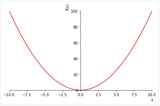
Following example plots values of x2 for each value in range(-10,10) −

>>> from sympy.plotting import plot 
>>> from sympy import * 
>>> x=Symbol('x') 
>>> plot(x**2, line_color='red')

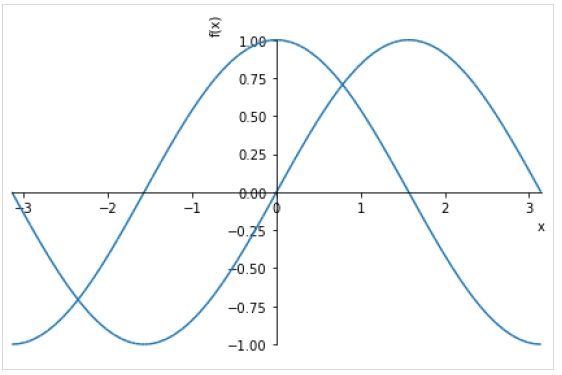
To draw multiple plots for same range, give multiple expressions prior to the range tuple.

>>> plot( sin(x),cos(x), (x, -pi, pi))

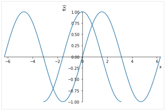
You can also specify separate range for each expression.

plot((expr1, range1), (expr2, range2))

Following figure plots sin(x) and cos(x) over different ranges.

>>> plot( (sin(x),(x, -2*pi, 2*pi)),(cos(x), (x, -pi, pi)))

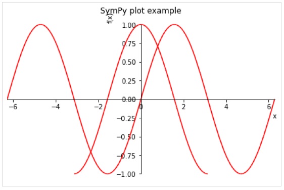
Following optional keyword arguments may be specified in plot() function.

• line_color − specifies color of the plot line.

• title − a string to be displayed as title

• xlabel − a string to be displayed as label for X axis

• ylabel − a string to be displayed as label for y axis

>>> plot( (sin(x),(x, -2*pi, 2*pi)),(cos(x), (x, -pi, pi)), line_color='red', title='SymPy plot example')

The plot3d() function renders a three dimensional plot.

plot3d(expr, xrange, yrange, kwargs)

Following example draws a 3D surface plot −

>>> from sympy.plotting import plot3d 
>>> x,y=symbols('x y') 
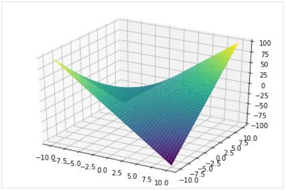
>>> plot3d(x*y, (x, -10,10), (y, -10,10))

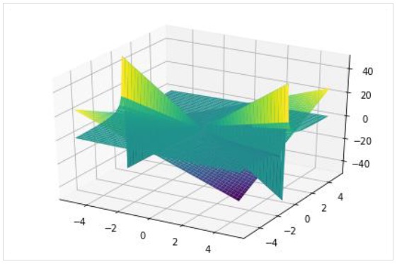
As in 2D plot, a three dimensional plot can also have multiple plots each with different range.

>>> plot3d(x*y, x/y, (x, -5, 5), (y, -5, 5))

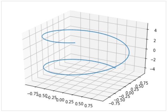
The plot3d_parametric_line() function renders a 3 dimensional parametric line plot.

>>> from sympy.plotting import plot3d_parametric_line 
>>> plot3d_parametric_line(cos(x), sin(x), x, (x, -5, 5))

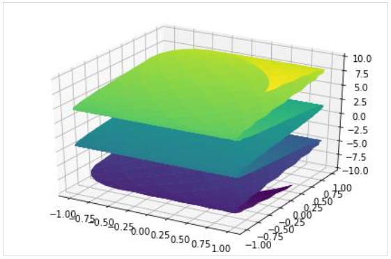
To draw a parametric surface plot, use plot3d_parametric_surface() function.

plot3d_parametric_surface(xexpr, yexpr, zexpr, rangex, rangey, kwargs)

>>> from sympy.plotting import plot3d_parametric_surface 
>>> plot3d_parametric_surface(cos(x+y), sin(x-y), x-y, (x, -5, 5), (y, -5, 5))

SymPy - Entities

The geometry module in SymPy allows creation of two dimensional entities such as line, circle, etc. We can then obtain information about them such as checking colinearity or finding intersection.

Point

Point class represents a point in Euclidean space. Following example checks for collinearity of points −

>>> from sympy.geometry import Point 
>>> from sympy import * 
>>> x=Point(0,0) 
>>> y=Point(2,2) 
>>> z=Point(4,4) 
>>> Point.is_collinear(x,y,z)

Output

True

>>> a=Point(2,3) 
>>> Point.is_collinear(x,y,a)

Output

False

The distance() method of Point class calculates distance between two points

>>> x.distance(y)

Output

$2\sqrt2$

The distance may also be represented in terms of symbols.

Line

Line entity is obtained from two Point objects. The intersection() method returns point of intersection if two lines intersect each other.

>>> from sympy.geometry import Point, Line 
>>> p1, p2=Point(0,5), Point(5,0) 
>>> l1=Line(p1,p2)
>>> l2=Line(Point(0,0), Point(5,5)) 
>>> l1.intersection(l2)

Output

[Point2D(5/2, 5/2)]

>>> l1.intersection(Line(Point(0,0), Point(2,2)))

Output

[Point2D(5/2, 5/2)]

>>> x,y=symbols('x y') 
>>> p=Point(x,y) 
>>> p.distance(Point(0,0))

Output

$\sqrt{x^2 + y^2}$

Triangle

This function builds a triangle entity from three point objects.

Triangle(a,b,c)

>>> t=Triangle(Point(0,0),Point(0,5), Point(5,0)) 
>>> t.area

Output

$-\frac{25}{2}$

Ellipse

An elliptical geometry entity is constructed by passing a Point object corresponding to center and two numbers each for horizontal and vertical radius.

ellipse(center, hradius, vradius)

>>> from sympy.geometry import Ellipse, Line 
>>> e=Ellipse(Point(0,0),8,3) 
>>> e.area

Output

$24\pi$

The vradius can be indirectly provided by using eccentricity parameter.

>>> e1=Ellipse(Point(2,2), hradius=5, eccentricity=Rational(3,4)) 
>>> e1.vradius

Output

$\frac{5\sqrt7}{4}$

The apoapsis of the ellipse is the greatest distance between the focus and the contour.

>>> e1.apoapsis

Output

$\frac{35}{4}$

Following statement calculates circumference of ellipse −

>>> e1.circumference

Output

$20E(\frac{9}{16})$

The equation method of ellipse returns equation of ellipse.

>>> e1.equation(x,y)

Output

$(\frac{x}{5}-\frac{2}{5})^2 + \frac{16(y-2)2}{175} - 1$

SymPy - Sets

In mathematics, a set is a well-defined collection of distinct objects which may be numbers, people, letters of the alphabet, or even other sets. Set is also one of the built-in types in Python. SymPy provides sets module. It contains definitions of different types of set and has functionality to perform set operations such as intersection, union, etc.

Set is a base class for any other type of set in SymPy. Note that it is different from built-in set data type of Python. Interval class represents real intervals and its boundary property returns a FiniteSet object.

>>> from sympy import Interval 
>>> s=Interval(1,10).boundary 
>>> type(s)

sympy.sets.sets.FiniteSet

FiniteSet is a collection of discrete numbers. It can be obtained from any sequence object such as list or string.

>>> from sympy import FiniteSet 
>>> FiniteSet(range(5))

Output

$\lbrace\lbrace0,1,...,4\rbrace\rbrace$

>>> numbers=[1,3,5,2,8] 
>>> FiniteSet(*numbers)

Output

$\lbrace1,2,3,5,8\rbrace$

>>> s="HelloWorld" 
>>> FiniteSet(*s)

Output

{H,W,d,e,l,o,r}

Note that, as in built-in set, SymPy's Set is also a collection of distinct objects.

ConditionSet is a set of elements that satisfy a given condition

>>> from sympy import ConditionSet, Eq, Symbol 
>>> x=Symbol('x') 
>>> s=ConditionSet(x, Eq(x**2-2*x,0), Interval(1,10)) >>> s

Output

$\lbrace x\mid x\in[1,10]∧x^2 - 2x =0\rbrace$

Union is a compound set. It includes all elements in two sets. Note that elements that are found in both, will appear only once in the Union.

>>> from sympy import Union 
>>> l1=[3,1,5,7] 
>>> l2=[9,7,2,1] 
>>> a=FiniteSet(*l1) 
>>> b=FiniteSet(*l2) 
>>> Union(a,b)

Intersection on the other hand contains only those elements that are present in both.

>>> from sympy import Intersection 
>>> Intersection(a,b)

ProductSet object represents Cartesian product of elements in both sets.

>>> from sympy import ProductSet 
>>> l1=[1,2] 
>>> l2=[2,3] 
>>> a=FiniteSet(*l1) 
>>> b=FiniteSet(*l2) 
>>> set(ProductSet(a,b))

Complement(a,b) retains elements in a excluding elements that are common with b set.

>>> from sympy import Complement 
>>> l1=[3,1,5,7] 
>>> l2=[9,7,2,1] 
>>> a=FiniteSet(*l1) 
>>> b=FiniteSet(*l2) 
>>> Complement(a,b), Complement(b,a)

SymmetricDifference set contains only uncommon elements in both sets.

>>> from sympy import SymmetricDifference 
>>> l1=[3,1,5,7] 
>>> l2=[9,7,2,1] 
>>> a=FiniteSet(*l1) 
>>> b=FiniteSet(*l2) 
>>> SymmetricDifference(a,b)

Output

{2,3,5,9}

SymPy - Printing

There are several printers available in SymPy. Following is a partial list −

• str
• srepr
• ASCII pretty printer
• Unicode pretty printer
• LaTeX
• MathML
• Dot

SymPy objects can also be sent as output to code of various languages, such as C, Fortran, Javascript, Theano, and Python.

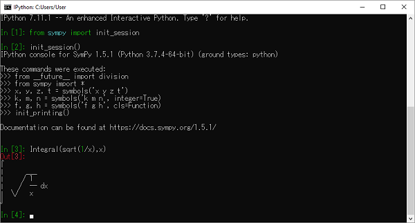
SymPy uses Unicode characters to render output in form of pretty print. If you are using Python console for executing SymPy session, the best pretty printing environment is activated by calling init_session() function.

>>> from sympy import init_session 
>>> init_session()

IPython console for SymPy 1.5.1 (Python 3.7.4-64-bit) (ground types: python).

These commands were executed −

>>> from __future__ import division
>>> from sympy import *
>>> x, y, z, t = symbols('x y z t')
>>> k, m, n = symbols('k m n', integer=True)
>>> f, g, h = symbols('f g h', cls=Function)
>>> init_printing()

Documentation can be found at https://docs.sympy.org/1.5.1/.

>>> Integral(sqrt(1/x),x)

$\int \sqrt\frac{1}{x} dx$

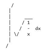
If LATEX is not installed, but Matplotlib is installed, it will use the Matplotlib rendering engine. If Matplotlib is not installed, it uses the Unicode pretty printer. However, Jupyter notebook uses MathJax to render LATEX.

In a terminal that does not support Unicode, ASCII pretty printer is used.

To use ASCII printer use pprint() function with use_unicode property set to False

>>> pprint(Integral(sqrt(1/x),x),use_unicode=False)

The Unicode pretty printer is also accessed from pprint() and pretty(). If the terminal supports Unicode, it is used automatically. If pprint() is not able to detect that the terminal supports unicode, you can pass use_unicode=True to force it to use Unicode.

To get the LATEX form of an expression, use latex() function.

>>> print(latex(Integral(sqrt(1/x),x)))

\int \sqrt{\frac{1}{x}}\, dx

You can also use mathml printer. for that purpose, import print_mathml function. A string version is obtained by mathml() function.

>>> from sympy.printing.mathml import print_mathml 
>>> print_mathml(Integral(sqrt(1/x),x))

<apply>

<int/>

<bvar>

<ci>x</ci>

</bvar>

<apply>

<root/>

<apply>

<power/>

<ci>x</ci>

<cn>-1</cn>

</apply>

</apply>

</apply>

>>>mathml(Integral(sqrt(1/x),x))

'<apply><int/><bvar><ci>x</ci></bvar><apply><root/><apply><power/><ci>x</ci><cn>-1</cn></apply></apply></apply>'