- Scikit Learn - Home
- Scikit Learn - Introduction
- Scikit Learn - Modelling Process
- Scikit Learn - Data Representation
- Scikit Learn - Estimator API
- Scikit Learn - Conventions
- Scikit Learn - Linear Modeling
- Scikit Learn - Extended Linear Modeling
- Stochastic Gradient Descent
- Scikit Learn - Support Vector Machines
- Scikit Learn - Anomaly Detection
- Scikit Learn - K-Nearest Neighbors
- Scikit Learn - KNN Learning
- Classification with Naïve Bayes
- Scikit Learn - Decision Trees
- Randomized Decision Trees
- Scikit Learn - Boosting Methods
- Scikit Learn - Clustering Methods
- Clustering Performance Evaluation
- Dimensionality Reduction using PCA
- Scikit Learn Useful Resources
- Scikit Learn - Quick Guide
- Scikit Learn - Useful Resources
- Scikit Learn - Discussion
Scikit Learn - Estimator API
In this chapter, we will learn about Estimator API (application programming interface). Let us begin by understanding what is an Estimator API.
What is Estimator API
It is one of the main APIs implemented by Scikit-learn. It provides a consistent interface for a wide range of ML applications thats why all machine learning algorithms in Scikit-Learn are implemented via Estimator API. The object that learns from the data (fitting the data) is an estimator. It can be used with any of the algorithms like classification, regression, clustering or even with a transformer, that extracts useful features from raw data.
For fitting the data, all estimator objects expose a fit method that takes a dataset shown as follows −
estimator.fit(data)
Next, all the parameters of an estimator can be set, as follows, when it is instantiated by the corresponding attribute.
estimator = Estimator (param1=1, param2=2)
estimator.param1
The output of the above would be 1.
Once data is fitted with an estimator, parameters are estimated from the data at hand. Now, all the estimated parameters will be the attributes of the estimator object ending by an underscore as follows −
estimator.estimated_param_
Use of Estimator API
Main uses of estimators are as follows −
Estimation and decoding of a model
Estimator object is used for estimation and decoding of a model. Furthermore, the model is estimated as a deterministic function of the following −
The parameters which are provided in object construction.
The global random state (numpy.random) if the estimators random_state parameter is set to none.
Any data passed to the most recent call to fit, fit_transform, or fit_predict.
Any data passed in a sequence of calls to partial_fit.
Mapping non-rectangular data representation into rectangular data
It maps a non-rectangular data representation into rectangular data. In simple words, it takes input where each sample is not represented as an array-like object of fixed length, and producing an array-like object of features for each sample.
Distinction between core and outlying samples
It models the distinction between core and outlying samples by using following methods −
fit
fit_predict if transductive
predict if inductive
Guiding Principles
While designing the Scikit-Learn API, following guiding principles kept in mind −
Consistency
This principle states that all the objects should share a common interface drawn from a limited set of methods. The documentation should also be consistent.
Limited object hierarchy
This guiding principle says −
Algorithms should be represented by Python classes
Datasets should be represented in standard format like NumPy arrays, Pandas DataFrames, SciPy sparse matrix.
Parameters names should use standard Python strings.
Composition
As we know that, ML algorithms can be expressed as the sequence of many fundamental algorithms. Scikit-learn makes use of these fundamental algorithms whenever needed.
Sensible defaults
According to this principle, the Scikit-learn library defines an appropriate default value whenever ML models require user-specified parameters.
Inspection
As per this guiding principle, every specified parameter value is exposed as pubic attributes.
Steps in using Estimator API
Followings are the steps in using the Scikit-Learn estimator API −
Step 1: Choose a class of model
In this first step, we need to choose a class of model. It can be done by importing the appropriate Estimator class from Scikit-learn.
Step 2: Choose model hyperparameters
In this step, we need to choose class model hyperparameters. It can be done by instantiating the class with desired values.
Step 3: Arranging the data
Next, we need to arrange the data into features matrix (X) and target vector(y).
Step 4: Model Fitting
Now, we need to fit the model to your data. It can be done by calling fit() method of the model instance.
Step 5: Applying the model
After fitting the model, we can apply it to new data. For supervised learning, use predict() method to predict the labels for unknown data. While for unsupervised learning, use predict() or transform() to infer properties of the data.
Supervised Learning Example
Here, as an example of this process we are taking common case of fitting a line to (x,y) data i.e. simple linear regression.
First, we need to load the dataset, we are using iris dataset −
Example
import seaborn as sns
iris = sns.load_dataset('iris')
X_iris = iris.drop('species', axis = 1)
X_iris.shape
Output
(150, 4)
Example
y_iris = iris['species']
y_iris.shape
Output
(150,)
Example
Now, for this regression example, we are going to use the following sample data −
%matplotlib inline
import matplotlib.pyplot as plt
import numpy as np
rng = np.random.RandomState(35)
x = 10*rng.rand(40)
y = 2*x-1+rng.randn(40)
plt.scatter(x,y);
Output
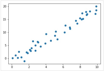
So, we have the above data for our linear regression example.
Now, with this data, we can apply the above-mentioned steps.
Choose a class of model
Here, to compute a simple linear regression model, we need to import the linear regression class as follows −
from sklearn.linear_model import LinearRegression
Choose model hyperparameters
Once we choose a class of model, we need to make some important choices which are often represented as hyperparameters, or the parameters that must set before the model is fit to data. Here, for this example of linear regression, we would like to fit the intercept by using the fit_intercept hyperparameter as follows −
Example
model = LinearRegression(fit_intercept = True)
model
Output
LinearRegression(copy_X = True, fit_intercept = True, n_jobs = None, normalize = False)
Arranging the data
Now, as we know that our target variable y is in correct form i.e. a length n_samples array of 1-D. But, we need to reshape the feature matrix X to make it a matrix of size [n_samples, n_features]. It can be done as follows −
Example
X = x[:, np.newaxis]
X.shape
Output
(40, 1)
Model fitting
Once, we arrange the data, it is time to fit the model i.e. to apply our model to data. This can be done with the help of fit() method as follows −
Example
model.fit(X, y)
Output
LinearRegression(copy_X = True, fit_intercept = True, n_jobs = None,normalize = False)
In Scikit-learn, the fit() process have some trailing underscores.
For this example, the below parameter shows the slope of the simple linear fit of the data −
Example
model.coef_
Output
array([1.99839352])
The below parameter represents the intercept of the simple linear fit to the data −
Example
model.intercept_
Output
-0.9895459457775022
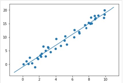
Applying the model to new data
After training the model, we can apply it to new data. As the main task of supervised machine learning is to evaluate the model based on new data that is not the part of the training set. It can be done with the help of predict() method as follows −
Example
xfit = np.linspace(-1, 11)
Xfit = xfit[:, np.newaxis]
yfit = model.predict(Xfit)
plt.scatter(x, y)
plt.plot(xfit, yfit);
Output
Complete working/executable example
%matplotlib inline
import matplotlib.pyplot as plt
import numpy as np
import seaborn as sns

iris = sns.load_dataset('iris')
X_iris = iris.drop('species', axis = 1)
X_iris.shape
y_iris = iris['species']
y_iris.shape

rng = np.random.RandomState(35)
x = 10*rng.rand(40)
y = 2*x-1+rng.randn(40)
plt.scatter(x,y);
from sklearn.linear_model import LinearRegression
model = LinearRegression(fit_intercept=True)
model
X = x[:, np.newaxis]
X.shape

model.fit(X, y)
model.coef_
model.intercept_

xfit = np.linspace(-1, 11)
Xfit = xfit[:, np.newaxis]
yfit = model.predict(Xfit)
plt.scatter(x, y)
plt.plot(xfit, yfit);
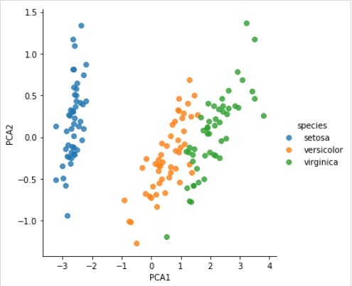
Unsupervised Learning Example
Here, as an example of this process we are taking common case of reducing the dimensionality of the Iris dataset so that we can visualize it more easily. For this example, we are going to use principal component analysis (PCA), a fast-linear dimensionality reduction technique.
Like the above given example, we can load and plot the random data from iris dataset. After that we can follow the steps as below −
Choose a class of model
from sklearn.decomposition import PCA
Choose model hyperparameters
Example
model = PCA(n_components=2)
model
Output
PCA(copy = True, iterated_power = 'auto', n_components = 2, random_state = None,
   svd_solver = 'auto', tol = 0.0, whiten = False)
Model fitting
Example
model.fit(X_iris)
Output
PCA(copy = True, iterated_power = 'auto', n_components = 2, random_state = None,
   svd_solver = 'auto', tol = 0.0, whiten = False)
Transform the data to two-dimensional
Example
X_2D = model.transform(X_iris)
Now, we can plot the result as follows −
Output
iris['PCA1'] = X_2D[:, 0]
iris['PCA2'] = X_2D[:, 1]
sns.lmplot("PCA1", "PCA2", hue = 'species', data = iris, fit_reg = False);
Output
Complete working/executable example
%matplotlib inline
import matplotlib.pyplot as plt
import numpy as np
import seaborn as sns

iris = sns.load_dataset('iris')
X_iris = iris.drop('species', axis = 1)
X_iris.shape
y_iris = iris['species']
y_iris.shape
rng = np.random.RandomState(35)
x = 10*rng.rand(40)
y = 2*x-1+rng.randn(40)
plt.scatter(x,y);
from sklearn.decomposition import PCA

model = PCA(n_components=2)
model
model.fit(X_iris)
X_2D = model.transform(X_iris)
iris['PCA1'] = X_2D[:, 0]
iris['PCA2'] = X_2D[:, 1]
sns.lmplot("PCA1", "PCA2", hue='species', data=iris, fit_reg=False);
