- R - Home
- R - Overview
- R - Environment Setup
- R - Basic Syntax
- R - Data Types
- R - Variables
- R - Operators
- R - Decision Making
- R - Loops
- R - Functions
- R - Strings
- R - Vectors
- R - Lists
- R - Matrices
- R - Arrays
- R - Factors
- R - Data Frames
- R - Packages
- R - Data Reshaping
- R - CSV Files
- R - Excel Files
- R - Binary Files
- R - XML Files
- R - JSON Files
- R - Web Data
- R - Database
- R Charts & Graphs
- R - Pie Charts
- R - Bar Charts
- R - Boxplots
- R - Histograms
- R - Line Graphs
- R - Scatterplots
- R Statistics Examples
- R - Mean, Median & Mode
- R - Linear Regression
- R - Multiple Regression
- R - Logistic Regression
- R - Normal Distribution
- R - Binomial Distribution
- R - Poisson Regression
- R - Analysis of Covariance
- R - Time Series Analysis
- R - Nonlinear Least Square
- R - Decision Tree
- R - Random Forest
- R - Survival Analysis
- R - Chi Square Tests
- R Useful Resources
- R - Interview Questions
- R - Quick Guide
- R - Cheatsheet
- R - Useful Resources
- R - Discussion
R - Survival Analysis
Survival analysis deals with predicting the time when a specific event is going to occur. It is also known as failure time analysis or analysis of time to death. For example predicting the number of days a person with cancer will survive or predicting the time when a mechanical system is going to fail.
The R package named survival is used to carry out survival analysis. This package contains the function Surv() which takes the input data as a R formula and creates a survival object among the chosen variables for analysis. Then we use the function survfit() to create a plot for the analysis.
Install Package
install.packages("survival")
Syntax
The basic syntax for creating survival analysis in R is −
Surv(time,event)
survfit(formula)
Following is the description of the parameters used −
time is the follow up time until the event occurs.
event indicates the status of occurrence of the expected event.
formula is the relationship between the predictor variables.
Example
We will consider the data set named "pbc" present in the survival packages installed above. It describes the survival data points about people affected with primary biliary cirrhosis (PBC) of the liver. Among the many columns present in the data set we are primarily concerned with the fields "time" and "status". Time represents the number of days between registration of the patient and earlier of the event between the patient receiving a liver transplant or death of the patient.
# Load the library.
library("survival")

# Print first few rows.
print(head(pbc))
When we execute the above code, it produces the following result and chart −
  id time status trt      age sex ascites hepato spiders edema bili chol
1  1  400      2   1 58.76523   f       1      1       1   1.0 14.5  261
2  2 4500      0   1 56.44627   f       0      1       1   0.0  1.1  302
3  3 1012      2   1 70.07255   m       0      0       0   0.5  1.4  176
4  4 1925      2   1 54.74059   f       0      1       1   0.5  1.8  244
5  5 1504      1   2 38.10541   f       0      1       1   0.0  3.4  279
6  6 2503      2   2 66.25873   f       0      1       0   0.0  0.8  248
  albumin copper alk.phos    ast trig platelet protime stage
1    2.60    156   1718.0 137.95  172      190    12.2     4
2    4.14     54   7394.8 113.52   88      221    10.6     3
3    3.48    210    516.0  96.10   55      151    12.0     4
4    2.54     64   6121.8  60.63   92      183    10.3     4
5    3.53    143    671.0 113.15   72      136    10.9     3
6    3.98     50    944.0  93.00   63       NA    11.0     3
From the above data we are considering time and status for our analysis.
Applying Surv() and survfit() Function
Now we proceed to apply the Surv() function to the above data set and create a plot that will show the trend.
# Load the library.
library("survival")

# Create the survival object.
survfit(Surv(pbc$time,pbc$status == 2)~1)

# Give the chart file a name.
png(file = "survival.png")

# Plot the graph.
plot(survfit(Surv(pbc$time,pbc$status == 2)~1))

# Save the file.
dev.off()
When we execute the above code, it produces the following result and chart −
Call: survfit(formula = Surv(pbc$time, pbc$status == 2) ~ 1)

      n  events  median 0.95LCL 0.95UCL
    418     161    3395    3090    3853
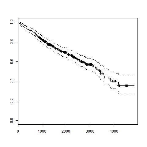
The trend in the above graph helps us predicting the probability of survival at the end of a certain number of days.
