PyTorch - Linear Regression

In this chapter, we will be focusing on basic example of linear regression implementation using TensorFlow. Logistic regression or linear regression is a supervised machine learning approach for the classification of order discrete categories. Our goal in this chapter is to build a model by which a user can predict the relationship between predictor variables and one or more independent variables.

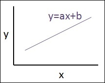
The relationship between these two variables is considered linear i.e., if y is the dependent variable and x is considered as the independent variable, then the linear regression relationship of two variables will look like the equation which is mentioned as below −

Y = Ax+b

Next, we shall design an algorithm for linear regression which allows us to understand two important concepts given below −

• Cost Function
• Gradient Descent Algorithms

The schematic representation of linear regression is mentioned below

Interpreting the result

$$Y=ax+b$$

• The value of a is the slope.

• The value of b is the y − intercept.

• r is the correlation coefficient.

• r² is the correlation coefficient.

The graphical view of the equation of linear regression is mentioned below −

Following steps are used for implementing linear regression using PyTorch −

Step 1

Import the necessary packages for creating a linear regression in PyTorch using the below code −

import numpy as np
import matplotlib.pyplot as plt
from matplotlib.animation import FuncAnimation
import seaborn as sns
import pandas as pd
%matplotlib inline

sns.set_style(style = 'whitegrid')
plt.rcParams["patch.force_edgecolor"] = True

Step 2

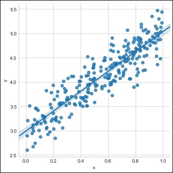
Create a single training set with the available data set as shown below −

m = 2 # slope
c = 3 # interceptm = 2 # slope
c = 3 # intercept
x = np.random.rand(256)

noise = np.random.randn(256) / 4

y = x * m + c + noise

df = pd.DataFrame()
df['x'] = x
df['y'] = y

sns.lmplot(x ='x', y ='y', data = df)

Step 3

Implement linear regression with PyTorch libraries as mentioned below −

import torch
import torch.nn as nn
from torch.autograd import Variable
x_train = x.reshape(-1, 1).astype('float32')
y_train = y.reshape(-1, 1).astype('float32')

class LinearRegressionModel(nn.Module):
   def __init__(self, input_dim, output_dim):
      super(LinearRegressionModel, self).__init__()
      self.linear = nn.Linear(input_dim, output_dim)

   def forward(self, x):
      out = self.linear(x)
      return out
input_dim = x_train.shape[1]
output_dim = y_train.shape[1]
input_dim, output_dim(1, 1)
model = LinearRegressionModel(input_dim, output_dim)
criterion = nn.MSELoss()
[w, b] = model.parameters()

def get_param_values():
   return w.data[0][0], b.data[0]

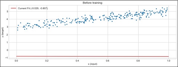
def plot_current_fit(title = ""):
plt.figure(figsize = (12,4))
plt.title(title)
plt.scatter(x, y, s = 8)
w1 = w.data[0][0]
b1 = b.data[0]
x1 = np.array([0., 1.])
y1 = x1 * w1 + b1
plt.plot(x1, y1, 'r', label = 'Current Fit ({:.3f}, {:.3f})'.format(w1, b1))
plt.xlabel('x (input)')
plt.ylabel('y (target)')
plt.legend()
plt.show()
plot_current_fit('Before training')

The plot generated is as follows −