- Prophet - Home
- Prophet - Introduction
- Prophet - Basics of Time Series
- Prophet - Environment Setup
- Prophet - Installation
- Prophet - Installation in R
- Prophet - Getting Started
- Prophet Fundamentals
- Prophet - Data Preparation
- Prophet Useful Resources
- Prophet - Useful Resources
- Prophet - Discussion
Python Prophet - Getting Started
Prophet is a Python library for time series forecasting that automatically handles trends, seasonality, and missing data. It covers the complete workflow for getting started, including preparing data, fitting the model, generating forecasts, visualizing results, and saving predictions.
Understanding the Prophet Workflow
The Prophet model is designed for easy time series forecasting. It automatically handles trends, seasonality, and missing data with minimal configuration. The forecasting process is simple and follows these steps −
- The first step is to prepare the time series data in the required format.
- The second step is to initialize the Prophet model.
- The third step is to fit the model to the historical data.
- The fourth step is to create a future dataframe to define the forecast horizon.
- The fifth step is to generate the forecasts.
- And the final step is to visualize and interpret the results.
Prophet's Required Data Format
Prophet requires the dataset to be in a structured format with exactly two columns −
- ds − This is the date or timestamp column (stands for "datestamp").
- Y − This is the numeric value to forecast.
The column names must be exactly "ds" and "y". Prophet will not work with columns named "date" or "value".
The ds column can accept various date formats like '2020-01-01', '2020-01-01 14:30:00', or Unix timestamps. The y column contains numeric values for forecasting, such as sales numbers, website visits, or temperatures.
The timestamps must be valid and in chronological order. Missing dates are allowed, and Prophet handles gaps automatically.
Here's an example of the required structure −
| ds | y |
|---|---|
| 2021-01-01 | 123 |
| 2021-01-02 | 150 |
| 2021-01-03 | 98 |
Creating the First Dataset in Python
To get started with Prophet, the first step is to create a dataset in the required format. In this example, daily sales for a full year are created, including trend, weekly seasonality, and random noise for realism.
First, import the necessary libraries −
import pandas as pd
import numpy as np
Here, pandas is used to handle data, and numpy is used for numerical operations such as generating random numbers.
Next, generate a date range for the entire year 2023 −
dates = pd.date_range(start='2023-01-01', end='2023-12-31', freq='D')
This generates a list of dates from January 1 to December 31, 2023, with daily intervals.
Now, create the sales data.
np.random.seed(42)
trend = np.linspace(100, 150, len(dates))
seasonality = 20 * np.sin(np.arange(len(dates)) * 2 * np.pi / 7)
noise = np.random.normal(0, 5, len(dates))
sales = trend + seasonality + noise
Here, trend represents a gradual increase in sales, seasonality is the repeating weekly pattern in sales and noise is the random variation added to the data.
Finally, create a DataFrame with the dates and sales data. The ds column will hold the dates, and the y column will hold the sales values.
df = pd.DataFrame({'ds': dates, 'y': sales})
print(df.head())
Following is the output after running the code.
          ds           y
0 2023-01-01  102.483571
1 2023-01-02  115.082671
2 2023-01-03  123.011726
3 2023-01-04  116.704912
4 2023-01-05   90.701009
Initializing and Fitting the Prophet Model
Now that the dataset is prepared, the next step is to create a Prophet model and fit it to the data. First, import Prophet −
from prophet import Prophet
Then, create the Prophet model −
model = Prophet()
If an error occurs, uninstall the old version by running pip uninstall prophet and reinstall the new version by running pip install prophet.
Next, fit the model to the dataset that created earlier −
model.fit(df)
Creating Future Dates for Forecasting
Before making predictions, Prophet needs the information on how far into the future to forecast. A list of future dates is created using the make_future_dataframe function. For example, to forecast 90 days into the future, use the following −
future = model.make_future_dataframe(periods=90)
print(future.tail())
Generating Predictions
Once the future dates are ready, use the predict method to generate forecasts −
forecast = model.predict(future)
print(forecast[['ds', 'yhat', 'yhat_lower', 'yhat_upper']].tail())
This gives the predicted values (yhat) along with their lower and upper bounds (yhat_lower and yhat_upper).
After running the command, You will see the following output −
            ds        yhat  yhat_lower  yhat_upper
450 2024-03-26  180.776435  174.862981  186.764119
451 2024-03-27  171.161638  165.014731  176.792737
452 2024-03-28  153.311795  147.210514  159.180881
453 2024-03-29  143.098987  137.143426  149.134078
454 2024-03-30  147.461709  141.532230  153.979530
Visualizing the Forecast
To visualize the forecast, Prophet has a built-in plotting function. First, import matplotlib to create the plot. Then, use the following code to generate the visualization.
import matplotlib.pyplot as plt
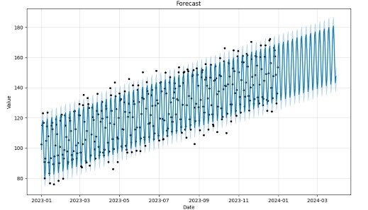
fig = model.plot(forecast)
plt.title('Forecast')
plt.xlabel('Date')
plt.ylabel('Value')
plt.show()
This plot shows the historical data alongside the forecasted values. The shaded area represents the range in which future values are likely to fall, reflecting the model's uncertainty in its predictions.
Visualizing Forecast Components
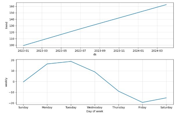
Prophet breaks the forecast into trend and seasonal components, making it easy to see how each part affects the predictions. The plot_components function of the model is used to create the graph, and plt.show() displays it.
fig2 = model.plot_components(forecast)
plt.show()
This creates separate plots showing trend which is the overall direction (upward, downward, or flat) and the weekly pattern (which days are higher or lower). Below is the output graph.
Below is the graph showing the long-term trend and seasonal cycles, such as weekly or yearly patterns. graph
Filtering Only Future Predictions
The forecast can be filtered to keep only future dates beyond the historical data, showing predicted values along with their lower and upper bounds.
future_predictions = forecast[forecast['ds'] > df['ds'].max()]
print(future_predictions[['ds', 'yhat', 'yhat_lower', 'yhat_upper']].head())
The output gives a clear view of upcoming predictions without including past data.
            ds        yhat  yhat_lower  yhat_upper
365 2024-01-01  166.784287  160.628995  172.777860
366 2024-01-02  169.256622  163.276815  175.819721
367 2024-01-03  159.641825  153.648941  165.565299
368 2024-01-04  141.791982  135.316069  147.882443
369 2024-01-05  131.579174  126.007299  137.371299
Saving the Forecast
The forecast can be saved to a CSV file using the to_csv() function. It can be saved as a full CSV containing all data or as a CSV containing only the date, predicted values, and their lower and upper uncertainty bounds.
# Save the full forecast with all columns
forecast.to_csv('sales_forecast.csv', index=False)

# Save only the key columns: date, predicted value, and uncertainty bounds
forecast[['ds', 'yhat', 'yhat_lower', 'yhat_upper']].to_csv('sales_forecast_simple.csv', index=False)
Conclusion
In this chapter, we learned how to use Prophet for accurate time series forecasting. By preparing data, fitting the model, making predictions, and looking at trends and patterns, it is easy to understand the data better. Prophet makes forecasting simple and easy to use.
