Selected Reading

Data Preparation in Python Prophet

Quiz

Data preparation in Prophet means turning raw time-series data into a clean and structured format. This includes correcting date formats, cleaning the target values, and handling missing or incorrect entries.

It also involves fixing irregular timestamps through resampling and preparing any features Prophet needs. The aim is to provide a clear, consistent timeline so the model can learn patterns accurately.

Inspect and Understand the Raw Time Series

The first step in data preparation is to load the dataset and see what the data looks like. For that we have downloaded the sales dataset from Kaggle.

import pandas as pd
import numpy as np

df = pd.read_csv("sales.csv")
print(df.head())
print(df.info())
print(df.describe())

Once it loads, we check if the date column is correct, the values are numeric, and the timestamps follow a regular pattern. These checks help us understand what needs to be cleaned before using Prophet. Below is the output we get.

         data              sales    stock   price
0  01-01-2014      0   4972    1.29
1  02-01-2014     70   4902    1.29
2  03-01-2014     59   4843    1.29
3  04-01-2014     93   4750    1.29
4  05-01-2014     96   4654    1.29

Convert and Clean the Date Column

Prophet needs the date column to be in proper datetime format. We change it so the dates are readable and Prophet can work with them correctly.

df['data'] = pd.to_datetime(df['data'])

If the automatic conversion does not match the file's format, we provide the correct date pattern −

df['data'] = pd.to_datetime(df['data'], format='%d-%m-%Y')

Clean the Target Variable

The target column , sales, must contain only numeric values. In many datasets, entries may include symbols, commas, currency signs, or empty strings, such as "$1,200", "3,500", or " ". To fix this, we remove all symbols and formatting from the column −

df['sales'] = df['sales'].astype(str).str.replace(r'[\$,]', '', regex=True)

After removing these characters, we convert the column into numeric values −

df['sales'] = pd.to_numeric(df['sales'], errors='coerce')

Then we display the first few rows to confirm that the values are now clean.

print(df['sales'].head())

Following is the output which displays the cleaned numeric values in the sales column −

0     0
1    70
2    59
3    93
4    96
Name: sales, dtype: int64

Handle Missing Values

Prophet cannot train a model if the target column contains missing values. We will check for missing entries in each column by running the following command −

df.isnull().sum()

Filling Missing Values

Once we know there are missing values, we need to fill them carefully so we do not introduce values that distort the true trend.

Option 1: Forward Fill − Carry the last known value forward −

df['sales'] = df['sales'].fillna(method='ffill')

Option 2: Interpolation − Estimate missing values between known points −

df['sales'] = df['sales'].interpolate()

Choosing a Method

Select the method that best fits the given data −

Forward fill works well for data that changes slowly or for values that keep increasing over time, like cumulative counts.
Interpolation works well for continuous measures like daily sales amounts.

Finally, run the following code to verify that all missing values are handled −

df.isnull().sum()

Following is the output which displays that no missing values are left.

data     0
sales    0
stock    0
price    0
dtype: int64

Detect and Handle Outliers

Outliers are unusually high or low values that can throw off your model by stretching trends or seasonal patterns. Let's see how we can handle them.

Step 1: Visual Check

The first thing we can do is simply look at the data. We will plot the data to spot any unusual spikes or drops by running the following commands.

df.plot(x='data', y='sales', title='Sales Over Time')

Following graph displays the daily sales over time and shows the spikes, drops, and overall movement in the data.

Step 2: Detect Using IQR

The Interquartile Range (IQR) method helps find values that are much lower or higher than usual. Calculate the lower and upper bounds like this −

Q1 = df['sales'].quantile(0.25)
Q3 = df['sales'].quantile(0.75)
IQR = Q3 - Q1

lower = Q1 - 1.5 * IQR
upper = Q3 + 1.5 * IQR

Step 3: Clip Extreme Values

After finding the limits, clip any values outside the range so they don't throw off the model. To do this, use the clip method, which takes the lower and upper bounds as arguments and replaces values below or above them with the nearest limit.

df['sales'] = df['sales'].clip(lower, upper)

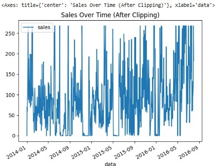
Now, we will print and plot the data to to visualize the changes −

#prints the data
print(df[['data', 'sales']].head())
#plots the graph
df.plot(x='data', y='sales', title='Sales Over Time (After Clipping)')

Below we can see the output, which displays the first few rows and the graph of our data.

        data  sales
0 2014-01-01      0
1 2014-01-02     70
2 2014-01-03     59
3 2014-01-04     93
4 2014-01-05     96

Resample the Time Series

Resampling is the process of changing the time frequency of a time series so that it has regular, evenly spaced intervals.

This is important because Prophet can only detect trends and patterns if the data has regular, consistent time intervals.

Resampling fixes this by filling in missing dates and combining data into fixed periods using an aggregation method. For example, to resample the data on a daily basis and calculate the average value for each day, the following code can be used −

df = df.set_index('data').resample('D').mean().reset_index()
print(df.head())

Following is the output, which shows the first few rows of the resampled data.

        data  sales   stock   price
0 2014-01-01    0.0  4972.0    1.29
1 2014-01-02   70.0  4902.0    1.29
2 2014-01-03   59.0  4843.0    1.29
3 2014-01-04   93.0  4750.0    1.29
4 2014-01-05   96.0  4654.0    1.29

Different aggregation methods can be used depending on the data types. For example −

sum() − for totals, such as daily sales or production counts.
mean() − for continuous measurements, like temperature or stock prices.
count() − for counting events.

Apply log Transform (Optional)

A log transform is useful when the values grow very fast or vary a lot. It reduces the scale of the numbers and makes the pattern smoother so Prophet can learn it better.

To apply the log transform, use the np.log() function. This function takes the natural log of each value in the column −

df['sales'] = np.log(df['sales'])
print(df.head())

Following is the output after applying the log transform.

       data     sales   stock   price
0 2014-01-01      -inf  4972.0    1.29
1 2014-01-02  4.248495  4902.0    1.29
2 2014-01-03  4.077537  4843.0    1.29
3 2014-01-04  4.532599  4750.0    1.29
4 2014-01-05  4.564348  4654.0    1.29

After forecasting, the values need to be brought back to the original scale. The np.exp() function reverses the log transform −

forecast['yhat'] = np.exp(forecast['yhat'])
print(forecast[['ds', 'yhat']].head())

Following is the output after reversing the log.

          ds        yhat
0 2014-01-01    0.0
1 2014-01-02   70.2
2 2014-01-03   58.7
3 2014-01-04   93.5
4 2014-01-05   96.1

Prepare Additional Regressors

Prophet can also use extra features that influence the target, like promotions, marketing spend, or weather. These features must be numeric, complete, and available for future dates.

For example, if the dataset has a promotion column, it can be converted to a numeric flag −

df['promo_flag'] = (df['promo'] == "Yes").astype(int)
print(df[['data', 'promo', 'promo_flag']].head())

Following is the output showing the first five rows with the promo_flag column, where 1 indicates a promotion and 0 means no promotion.

        data promo  promo_flag
0 2014-01-01    No           0
1 2014-01-02   Yes           1
2 2014-01-03    No           0
3 2014-01-04    No           0
4 2014-01-05   Yes           1

Split the Data into Training and Validation Sets

Since the model predicts future values based on past observations, we divide the data so that the training set contains earlier dates and the validation set contains later dates. This way, the model is tested on data it hasn't seen before.

train = df[df['data'] < '2024-09-01']
test = df[df['data'] >= '2024-09-01']

Final Clean Dataset

After all the cleaning and preparation, the dataset should have consistent dates, numeric target values, and optional regressors. To display the final cleaned dataset, run the following command −

print(df.head())

Following is the output that displays the cleaned dataset −

          ds      y  promo_flag
0   2024-01-01  200          0
1   2024-01-02  210          1
2   2024-01-03  220          0

Conclusion

In this chapter, we prepared the data for Prophet by fixing dates, handling missing or irregular values, and organizing everything into a consistent format. With these steps complete, the dataset is now ready for forecasting.

Previous Quiz Next