
Article Categories
- All Categories
-
 Data Structure
-
 Networking
-
 RDBMS
RDBMS
-
 Operating System
-
 Java
Java
-
 MS Excel
-
 iOS
iOS
-
 HTML
HTML
-
 CSS
CSS
-
 Android
-
 Python
-
 C Programming
-
 C++
C++
-
 C#
C#
-
 MongoDB
-
 MySQL
MySQL
-
 Javascript
-
 PHP
PHP
-
 Economics & Finance
Selected Reading
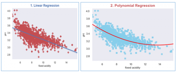
Plotting regression and residual plot in Matplotlib
To establish a simple relationship between the observations of a given joint distribution of a variable, we can create the plot for the regression model using Seaborn.
To fit the dataset using the regression model, we have to first import the necessary libraries in Python.
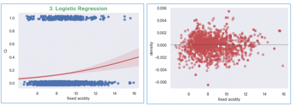
We will create plots for each regression model, (a) Linear Regression, (b) Polynomial Regression, and (c) Logistic Regression.
In this example, we will use the wine quality dataset which can be accessed from here, https://archive.ics.uci.edu/ml/datasets/wine+quality
Example
import matplotlib.pyplot as plt
import seaborn as sns
from scipy.stats import pearsonr
sns.set(style="dark", color_codes=True)

#import the dataset
wine_quality = pd.read_csv('winequality-red.csv', delimiter=';')

#Plotting Linear Regression
R, p = pearsonr(wine_quality['fixed acidity'], wine_quality.pH)
g1 = sns.regplot(x='fixed acidity', y='pH', data=wine_quality, truncate=True, ci=99,
marker='D', scatter_kws={'color': 'r'});
textstr = '$\mathrm{pearson}\hspace{0.5}\mathrm{R}^2=%.2f$<br>$\mathrm{pval}=%.2e$ '% (R**2, p)
props = dict(boxstyle='round', facecolor='wheat', alpha=0.5)
g1.text(0.55, 0.95, textstr, fontsize=14, va='top', bbox=props)
plt.title('1. Linear Regression', size=15, color='b', weight='bold')

#Let us Plot the Polynomial Regression plot for the wine dataset
g2 = sns.regplot(x='fixed acidity', y='pH', data=wine_quality, order=2, ci=None,
   marker='s', scatter_kws={'color': 'skyblue'},
   line_kws={'color': 'red'});
plt.title('2. Polynomial Regression', size=15, color='r', weight='bold')

#Now plotting the Logistic Regression
wine_quality['Q'] = wine_quality['quality'].map({'Low': 0, 'Med': 0, 'High':1})
g2 = sns.regplot(x='fixed acidity', y='Q', logistic=True,
   n_boot=750, y_jitter=.03, data=wine_quality,
   line_kws={'color': 'r'})
plt.show();

#Now plot the residual plot
g3 = sns.residplot(x='fixed acidity', y='density', order=2,
   data=wine_quality, scatter_kws={'color': 'r',
   'alpha': 0.5});
plt.show();
Running the above code will generate the output as,
Output

Updated on: 2021-02-23T18:14:13+05:30
2K+ Views

Advertisements