Selected Reading
Basis Path Testing
What is Basis Path Testing?
Basis path testing, a structured testing or white box testing technique used for designing test cases intended to examine all possible paths of execution at least once. Creating and executing tests for all possible paths results in 100% statement coverage and 100% branch coverage.
Example:
Function fn_delete_element (int value, int array_size, int array[])
{
	1 int i;
	location = array_size + 1;

	2 for i = 1 to array_size
	3 if ( array[i] == value )
	4 location = i;
	 end if;
	 end for;

	5 for i = location to array_size
	6 array[i] = array[i+1];
	end for;
	7 array_size --;
}
Steps to Calculate the independent paths
Step 1 : Draw the Flow Graph of the Function/Program under consideration as shown below:
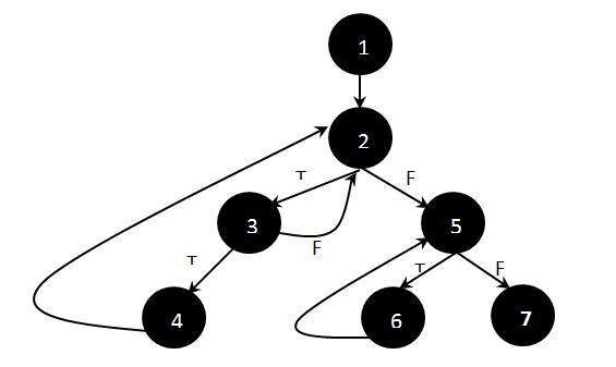
Step 2 : Determine the independent paths.
Path 1:  1 - 2 - 5 - 7
Path 2:  1 - 2 - 5 - 6 - 7
Path 3:  1 - 2 - 3 - 2 - 5 - 6 - 7
Path 4:  1 - 2 - 3 - 4 - 2 - 5 - 6 - 7

Advertisements