Parallel Algorithm - Quick Guide

---

---

Parallel Algorithm - Introduction

An algorithm is a sequence of steps that take inputs from the user and after some computation, produces an output. A parallel algorithm is an algorithm that can execute several instructions simultaneously on different processing devices and then combine all the individual outputs to produce the final result.

Concurrent Processing

The easy availability of computers along with the growth of Internet has changed the way we store and process data. We are living in a day and age where data is available in abundance. Every day we deal with huge volumes of data that require complex computing and that too, in quick time. Sometimes, we need to fetch data from similar or interrelated events that occur simultaneously. This is where we require concurrent processing that can divide a complex task and process it multiple systems to produce the output in quick time.

Concurrent processing is essential where the task involves processing a huge bulk of complex data. Examples include − accessing large databases, aircraft testing, astronomical calculations, atomic and nuclear physics, biomedical analysis, economic planning, image processing, robotics, weather forecasting, web-based services, etc.

What is Parallelism?

Parallelism is the process of processing several set of instructions simultaneously. It reduces the total computational time. Parallelism can be implemented by using parallel computers, i.e. a computer with many processors. Parallel computers require parallel algorithm, programming languages, compilers and operating system that support multitasking.

In this tutorial, we will discuss only about parallel algorithms. Before moving further, let us first discuss about algorithms and their types.

What is an Algorithm?

An algorithm is a sequence of instructions followed to solve a problem. While designing an algorithm, we should consider the architecture of computer on which the algorithm will be executed. As per the architecture, there are two types of computers −

• Sequential Computer
• Parallel Computer

Depending on the architecture of computers, we have two types of algorithms −

• Sequential Algorithm − An algorithm in which some consecutive steps of instructions are executed in a chronological order to solve a problem.

• Parallel Algorithm − The problem is divided into sub-problems and are executed in parallel to get individual outputs. Later on, these individual outputs are combined together to get the final desired output.

It is not easy to divide a large problem into sub-problems. Sub-problems may have data dependency among them. Therefore, the processors have to communicate with each other to solve the problem.

It has been found that the time needed by the processors in communicating with each other is more than the actual processing time. So, while designing a parallel algorithm, proper CPU utilization should be considered to get an efficient algorithm.

To design an algorithm properly, we must have a clear idea of the basic model of computation in a parallel computer.

Model of Computation

Both sequential and parallel computers operate on a set (stream) of instructions called algorithms. These set of instructions (algorithm) instruct the computer about what it has to do in each step.

Depending on the instruction stream and data stream, computers can be classified into four categories −

• Single Instruction stream, Single Data stream (SISD) computers
• Single Instruction stream, Multiple Data stream (SIMD) computers
• Multiple Instruction stream, Single Data stream (MISD) computers
• Multiple Instruction stream, Multiple Data stream (MIMD) computers

SISD Computers

SISD computers contain one control unit, one processing unit, and one memory unit.

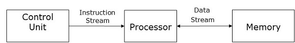
In this type of computers, the processor receives a single stream of instructions from the control unit and operates on a single stream of data from the memory unit. During computation, at each step, the processor receives one instruction from the control unit and operates on a single data received from the memory unit.

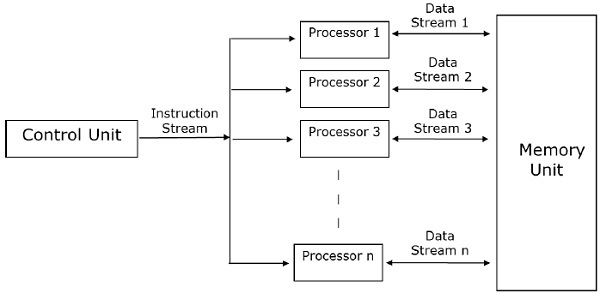
SIMD Computers

SIMD computers contain one control unit, multiple processing units, and shared memory or interconnection network.

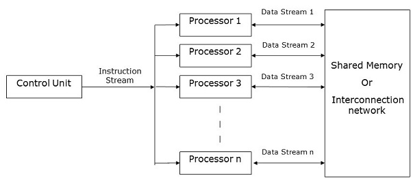
Here, one single control unit sends instructions to all processing units. During computation, at each step, all the processors receive a single set of instructions from the control unit and operate on different set of data from the memory unit.

Each of the processing units has its own local memory unit to store both data and instructions. In SIMD computers, processors need to communicate among themselves. This is done by shared memory or by interconnection network.

While some of the processors execute a set of instructions, the remaining processors wait for their next set of instructions. Instructions from the control unit decides which processor will be active (execute instructions) or inactive (wait for next instruction).

MISD Computers

As the name suggests, MISD computers contain multiple control units, multiple processing units, and one common memory unit.

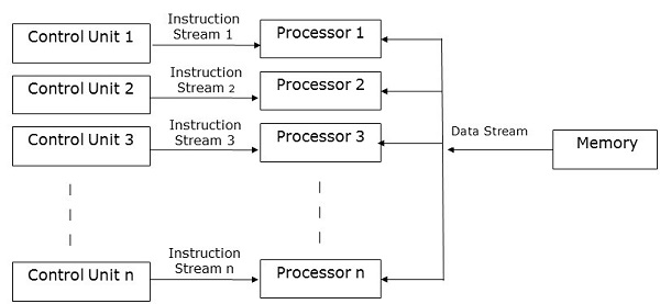
Here, each processor has its own control unit and they share a common memory unit. All the processors get instructions individually from their own control unit and they operate on a single stream of data as per the instructions they have received from their respective control units. This processor operates simultaneously.

MIMD Computers

MIMD computers have multiple control units, multiple processing units, and a shared memory or interconnection network.

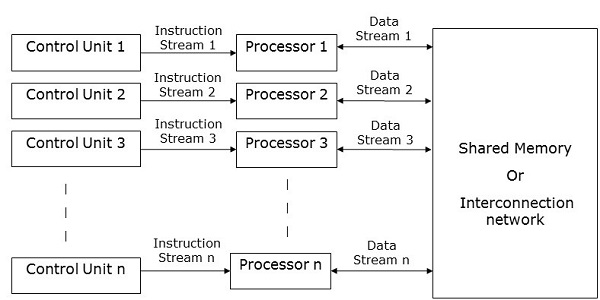
Here, each processor has its own control unit, local memory unit, and arithmetic and logic unit. They receive different sets of instructions from their respective control units and operate on different sets of data.

Note

• An MIMD computer that shares a common memory is known as multiprocessors, while those that uses an interconnection network is known as multicomputers.

• Based on the physical distance of the processors, multicomputers are of two types −

  • Multicomputer − When all the processors are very close to one another (e.g., in the same room).

  • Distributed system − When all the processors are far away from one another (e.g.- in the different cities)

Parallel Algorithm - Analysis

Analysis of an algorithm helps us determine whether the algorithm is useful or not. Generally, an algorithm is analyzed based on its execution time (Time Complexity) and the amount of space (Space Complexity) it requires.

Since we have sophisticated memory devices available at reasonable cost, storage space is no longer an issue. Hence, space complexity is not given so much of importance.

Parallel algorithms are designed to improve the computation speed of a computer. For analyzing a Parallel Algorithm, we normally consider the following parameters −

• Time complexity (Execution Time),
• Total number of processors used, and
• Total cost.

Time Complexity

The main reason behind developing parallel algorithms was to reduce the computation time of an algorithm. Thus, evaluating the execution time of an algorithm is extremely important in analyzing its efficiency.

Execution time is measured on the basis of the time taken by the algorithm to solve a problem. The total execution time is calculated from the moment when the algorithm starts executing to the moment it stops. If all the processors do not start or end execution at the same time, then the total execution time of the algorithm is the moment when the first processor started its execution to the moment when the last processor stops its execution.

Time complexity of an algorithm can be classified into three categories−

• Worst-case complexity − When the amount of time required by an algorithm for a given input is maximum.

• Average-case complexity − When the amount of time required by an algorithm for a given input is average.

• Best-case complexity − When the amount of time required by an algorithm for a given input is minimum.

Asymptotic Analysis

The complexity or efficiency of an algorithm is the number of steps executed by the algorithm to get the desired output. Asymptotic analysis is done to calculate the complexity of an algorithm in its theoretical analysis. In asymptotic analysis, a large length of input is used to calculate the complexity function of the algorithm.

Note − Asymptotic is a condition where a line tends to meet a curve, but they do not intersect. Here the line and the curve is asymptotic to each other.

Asymptotic notation is the easiest way to describe the fastest and slowest possible execution time for an algorithm using high bounds and low bounds on speed. For this, we use the following notations −

• Big O notation
• Omega notation
• Theta notation

Big O notation

In mathematics, Big O notation is used to represent the asymptotic characteristics of functions. It represents the behavior of a function for large inputs in a simple and accurate method. It is a method of representing the upper bound of an algorithm’s execution time. It represents the longest amount of time that the algorithm could take to complete its execution. The function −

f(n) = O(g(n))

iff there exists positive constants c and n₀ such that f(n) ≤ c * g(n) for all n where n ≥ n₀.

Omega notation

Omega notation is a method of representing the lower bound of an algorithm’s execution time. The function −

f(n) = Ω (g(n))

iff there exists positive constants c and n₀ such that f(n) ≥ c * g(n) for all n where n ≥ n₀.

Theta Notation

Theta notation is a method of representing both the lower bound and the upper bound of an algorithm’s execution time. The function −

f(n) = θ(g(n))

iff there exists positive constants c₁, c₂, and n₀ such that c1 * g(n) ≤ f(n) ≤ c2 * g(n) for all n where n ≥ n₀.

Speedup of an Algorithm

The performance of a parallel algorithm is determined by calculating its speedup. Speedup is defined as the ratio of the worst-case execution time of the fastest known sequential algorithm for a particular problem to the worst-case execution time of the parallel algorithm.

Number of Processors Used

The number of processors used is an important factor in analyzing the efficiency of a parallel algorithm. The cost to buy, maintain, and run the computers are calculated. Larger the number of processors used by an algorithm to solve a problem, more costly becomes the obtained result.

Total Cost

Total cost of a parallel algorithm is the product of time complexity and the number of processors used in that particular algorithm.

Total Cost = Time complexity × Number of processors used

Therefore, the efficiency of a parallel algorithm is −

Parallel Algorithm - Models

The model of a parallel algorithm is developed by considering a strategy for dividing the data and processing method and applying a suitable strategy to reduce interactions. In this chapter, we will discuss the following Parallel Algorithm Models −

• Data parallel model
• Task graph model
• Work pool model
• Master slave model
• Producer consumer or pipeline model
• Hybrid model

Data Parallel

In data parallel model, tasks are assigned to processes and each task performs similar types of operations on different data. Data parallelism is a consequence of single operations that is being applied on multiple data items.

Data-parallel model can be applied on shared-address spaces and message-passing paradigms. In data-parallel model, interaction overheads can be reduced by selecting a locality preserving decomposition, by using optimized collective interaction routines, or by overlapping computation and interaction.

The primary characteristic of data-parallel model problems is that the intensity of data parallelism increases with the size of the problem, which in turn makes it possible to use more processes to solve larger problems.

Example − Dense matrix multiplication.

Task Graph Model

In the task graph model, parallelism is expressed by a task graph. A task graph can be either trivial or nontrivial. In this model, the correlation among the tasks are utilized to promote locality or to minimize interaction costs. This model is enforced to solve problems in which the quantity of data associated with the tasks is huge compared to the number of computation associated with them. The tasks are assigned to help improve the cost of data movement among the tasks.

Examples − Parallel quick sort, sparse matrix factorization, and parallel algorithms derived via divide-and-conquer approach.

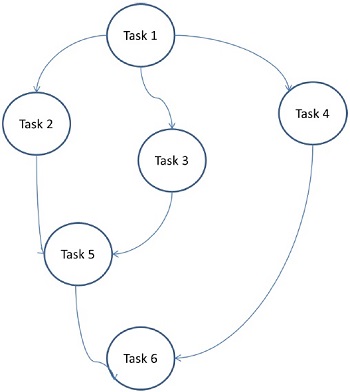
Here, problems are divided into atomic tasks and implemented as a graph. Each task is an independent unit of job that has dependencies on one or more antecedent task. After the completion of a task, the output of an antecedent task is passed to the dependent task. A task with antecedent task starts execution only when its entire antecedent task is completed. The final output of the graph is received when the last dependent task is completed (Task 6 in the above figure).

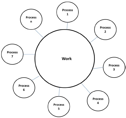
Work Pool Model

In work pool model, tasks are dynamically assigned to the processes for balancing the load. Therefore, any process may potentially execute any task. This model is used when the quantity of data associated with tasks is comparatively smaller than the computation associated with the tasks.

There is no desired pre-assigning of tasks onto the processes. Assigning of tasks is centralized or decentralized. Pointers to the tasks are saved in a physically shared list, in a priority queue, or in a hash table or tree, or they could be saved in a physically distributed data structure.

The task may be available in the beginning, or may be generated dynamically. If the task is generated dynamically and a decentralized assigning of task is done, then a termination detection algorithm is required so that all the processes can actually detect the completion of the entire program and stop looking for more tasks.

Example − Parallel tree search

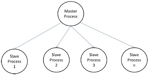
Master-Slave Model

In the master-slave model, one or more master processes generate task and allocate it to slave processes. The tasks may be allocated beforehand if −

• the master can estimate the volume of the tasks, or
• a random assigning can do a satisfactory job of balancing load, or
• slaves are assigned smaller pieces of task at different times.

This model is generally equally suitable to shared-address-space or message-passing paradigms, since the interaction is naturally two ways.

In some cases, a task may need to be completed in phases, and the task in each phase must be completed before the task in the next phases can be generated. The master-slave model can be generalized to hierarchical or multi-level master-slave model in which the top level master feeds the large portion of tasks to the second-level master, who further subdivides the tasks among its own slaves and may perform a part of the task itself.

Precautions in using the master-slave model

Care should be taken to assure that the master does not become a congestion point. It may happen if the tasks are too small or the workers are comparatively fast.

The tasks should be selected in a way that the cost of performing a task dominates the cost of communication and the cost of synchronization.

Asynchronous interaction may help overlap interaction and the computation associated with work generation by the master.

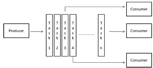
Pipeline Model

It is also known as the producer-consumer model. Here a set of data is passed on through a series of processes, each of which performs some task on it. Here, the arrival of new data generates the execution of a new task by a process in the queue. The processes could form a queue in the shape of linear or multidimensional arrays, trees, or general graphs with or without cycles.

This model is a chain of producers and consumers. Each process in the queue can be considered as a consumer of a sequence of data items for the process preceding it in the queue and as a producer of data for the process following it in the queue. The queue does not need to be a linear chain; it can be a directed graph. The most common interaction minimization technique applicable to this model is overlapping interaction with computation.

Example − Parallel LU factorization algorithm.

Hybrid Models

A hybrid algorithm model is required when more than one model may be needed to solve a problem.

A hybrid model may be composed of either multiple models applied hierarchically or multiple models applied sequentially to different phases of a parallel algorithm.

Example − Parallel quick sort

Parallel Random Access Machines

Parallel Random Access Machines (PRAM) is a model, which is considered for most of the parallel algorithms. Here, multiple processors are attached to a single block of memory. A PRAM model contains −

• A set of similar type of processors.

• All the processors share a common memory unit. Processors can communicate among themselves through the shared memory only.

• A memory access unit (MAU) connects the processors with the single shared memory.

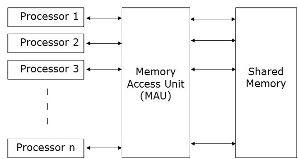
Here, n number of processors can perform independent operations on n number of data in a particular unit of time. This may result in simultaneous access of same memory location by different processors.

To solve this problem, the following constraints have been enforced on PRAM model −

• Exclusive Read Exclusive Write (EREW) − Here no two processors are allowed to read from or write to the same memory location at the same time.

• Exclusive Read Concurrent Write (ERCW) − Here no two processors are allowed to read from the same memory location at the same time, but are allowed to write to the same memory location at the same time.

• Concurrent Read Exclusive Write (CREW) − Here all the processors are allowed to read from the same memory location at the same time, but are not allowed to write to the same memory location at the same time.

• Concurrent Read Concurrent Write (CRCW) − All the processors are allowed to read from or write to the same memory location at the same time.

There are many methods to implement the PRAM model, but the most prominent ones are −

• Shared memory model
• Message passing model
• Data parallel model

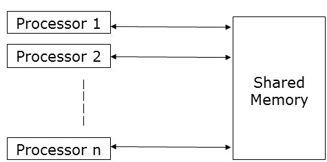
Shared Memory Model

Shared memory emphasizes on control parallelism than on data parallelism. In the shared memory model, multiple processes execute on different processors independently, but they share a common memory space. Due to any processor activity, if there is any change in any memory location, it is visible to the rest of the processors.

As multiple processors access the same memory location, it may happen that at any particular point of time, more than one processor is accessing the same memory location. Suppose one is reading that location and the other is writing on that location. It may create confusion. To avoid this, some control mechanism, like lock / semaphore, is implemented to ensure mutual exclusion.

Shared memory programming has been implemented in the following −

• Thread libraries − The thread library allows multiple threads of control that run concurrently in the same memory location. Thread library provides an interface that supports multithreading through a library of subroutine. It contains subroutines for

  • Creating and destroying threads
  • Scheduling execution of thread
  • passing data and message between threads
  • saving and restoring thread contexts

Examples of thread libraries include − SolarisTM threads for Solaris, POSIX threads as implemented in Linux, Win32 threads available in Windows NT and Windows 2000, and JavaTM threads as part of the standard JavaTM Development Kit (JDK).

• Distributed Shared Memory (DSM) Systems − DSM systems create an abstraction of shared memory on loosely coupled architecture in order to implement shared memory programming without hardware support. They implement standard libraries and use the advanced user-level memory management features present in modern operating systems. Examples include Tread Marks System, Munin, IVY, Shasta, Brazos, and Cashmere.

• Program Annotation Packages − This is implemented on the architectures having uniform memory access characteristics. The most notable example of program annotation packages is OpenMP. OpenMP implements functional parallelism. It mainly focuses on parallelization of loops.

The concept of shared memory provides a low-level control of shared memory system, but it tends to be tedious and erroneous. It is more applicable for system programming than application programming.

Merits of Shared Memory Programming

• Global address space gives a user-friendly programming approach to memory.

• Due to the closeness of memory to CPU, data sharing among processes is fast and uniform.

• There is no need to specify distinctly the communication of data among processes.

• Process-communication overhead is negligible.

• It is very easy to learn.

Demerits of Shared Memory Programming

• It is not portable.
• Managing data locality is very difficult.

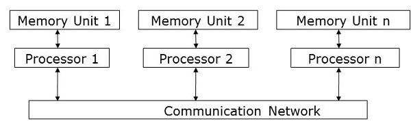
Message Passing Model

Message passing is the most commonly used parallel programming approach in distributed memory systems. Here, the programmer has to determine the parallelism. In this model, all the processors have their own local memory unit and they exchange data through a communication network.

Processors use message-passing libraries for communication among themselves. Along with the data being sent, the message contains the following components −

• The address of the processor from which the message is being sent;

• Starting address of the memory location of the data in the sending processor;

• Data type of the sending data;

• Data size of the sending data;

• The address of the processor to which the message is being sent;

• Starting address of the memory location for the data in the receiving processor.

Processors can communicate with each other by any of the following methods −

• Point-to-Point Communication
• Collective Communication
• Message Passing Interface

Point-to-Point Communication

Point-to-point communication is the simplest form of message passing. Here, a message can be sent from the sending processor to a receiving processor by any of the following transfer modes −

• Synchronous mode − The next message is sent only after the receiving a confirmation that its previous message has been delivered, to maintain the sequence of the message.

• Asynchronous mode − To send the next message, receipt of the confirmation of the delivery of the previous message is not required.

Collective Communication

Collective communication involves more than two processors for message passing. Following modes allow collective communications −

• Barrier − Barrier mode is possible if all the processors included in the communications run a particular bock (known as barrier block) for message passing.

• Broadcast − Broadcasting is of two types −

  • One-to-all − Here, one processor with a single operation sends same message to all other processors.

  • All-to-all − Here, all processors send message to all other processors.

Messages broadcasted may be of three types −

• Personalized − Unique messages are sent to all other destination processors.

• Non-personalized − All the destination processors receive the same message.

• Reduction − In reduction broadcasting, one processor of the group collects all the messages from all other processors in the group and combine them to a single message which all other processors in the group can access.

Merits of Message Passing

• Provides low-level control of parallelism;
• It is portable;
• Less error prone;
• Less overhead in parallel synchronization and data distribution.

Demerits of Message Passing

• As compared to parallel shared-memory code, message-passing code generally needs more software overhead.

Message Passing Libraries

There are many message-passing libraries. Here, we will discuss two of the most-used message-passing libraries −

• Message Passing Interface (MPI)
• Parallel Virtual Machine (PVM)

Message Passing Interface (MPI)

It is a universal standard to provide communication among all the concurrent processes in a distributed memory system. Most of the commonly used parallel computing platforms provide at least one implementation of message passing interface. It has been implemented as the collection of predefined functions called library and can be called from languages such as C, C++, Fortran, etc. MPIs are both fast and portable as compared to the other message passing libraries.

Merits of Message Passing Interface

• Runs only on shared memory architectures or distributed memory architectures;

• Each processors has its own local variables;

• As compared to large shared memory computers, distributed memory computers are less expensive.

Demerits of Message Passing Interface

• More programming changes are required for parallel algorithm;
• Sometimes difficult to debug; and
• Does not perform well in the communication network between the nodes.

Parallel Virtual Machine (PVM)

PVM is a portable message passing system, designed to connect separate heterogeneous host machines to form a single virtual machine. It is a single manageable parallel computing resource. Large computational problems like superconductivity studies, molecular dynamics simulations, and matrix algorithms can be solved more cost effectively by using the memory and the aggregate power of many computers. It manages all message routing, data conversion, task scheduling in the network of incompatible computer architectures.

Features of PVM

• Very easy to install and configure;
• Multiple users can use PVM at the same time;
• One user can execute multiple applications;
• It’s a small package;
• Supports C, C++, Fortran;
• For a given run of a PVM program, users can select the group of machines;
• It is a message-passing model,
• Process-based computation;
• Supports heterogeneous architecture.

Data Parallel Programming

The major focus of data parallel programming model is on performing operations on a data set simultaneously. The data set is organized into some structure like an array, hypercube, etc. Processors perform operations collectively on the same data structure. Each task is performed on a different partition of the same data structure.

It is restrictive, as not all the algorithms can be specified in terms of data parallelism. This is the reason why data parallelism is not universal.

Data parallel languages help to specify the data decomposition and mapping to the processors. It also includes data distribution statements that allow the programmer to have control on data – for example, which data will go on which processor – to reduce the amount of communication within the processors.

Parallel Algorithm - Structure

To apply any algorithm properly, it is very important that you select a proper data structure. It is because a particular operation performed on a data structure may take more time as compared to the same operation performed on another data structure.

Example − To access the i^th element in a set by using an array, it may take a constant time but by using a linked list, the time required to perform the same operation may become a polynomial.

Therefore, the selection of a data structure must be done considering the architecture and the type of operations to be performed.

The following data structures are commonly used in parallel programming −

• Linked List
• Arrays
• Hypercube Network

Linked List

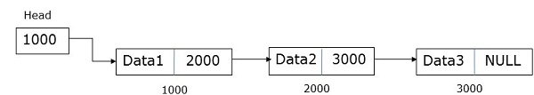
A linked list is a data structure having zero or more nodes connected by pointers. Nodes may or may not occupy consecutive memory locations. Each node has two or three parts − one data part that stores the data and the other two are link fields that store the address of the previous or next node. The first node’s address is stored in an external pointer called head. The last node, known as tail, generally does not contain any address.

There are three types of linked lists −

• Singly Linked List
• Doubly Linked List
• Circular Linked List

Singly Linked List

A node of a singly linked list contains data and the address of the next node. An external pointer called head stores the address of the first node.

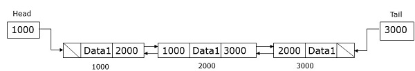
Doubly Linked List

A node of a doubly linked list contains data and the address of both the previous and the next node. An external pointer called head stores the address of the first node and the external pointer called tail stores the address of the last node.

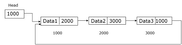
Circular Linked List

A circular linked list is very similar to the singly linked list except the fact that the last node saved the address of the first node.

Arrays

An array is a data structure where we can store similar types of data. It can be one-dimensional or multi-dimensional. Arrays can be created statically or dynamically.

• In statically declared arrays, dimension and size of the arrays are known at the time of compilation.

• In dynamically declared arrays, dimension and size of the array are known at runtime.

For shared memory programming, arrays can be used as a common memory and for data parallel programming, they can be used by partitioning into sub-arrays.

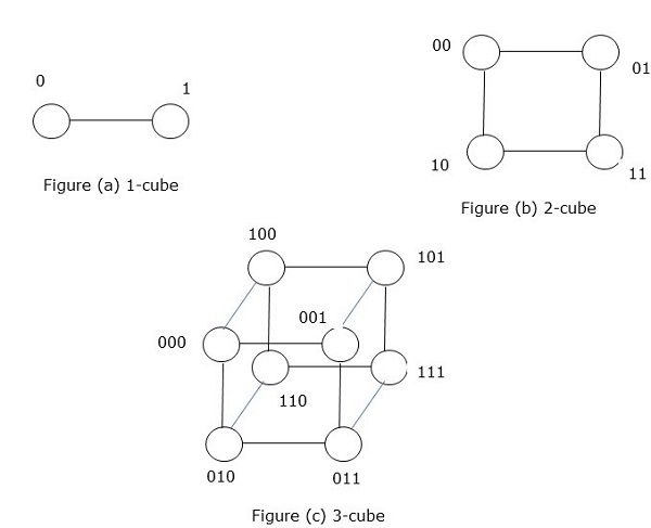
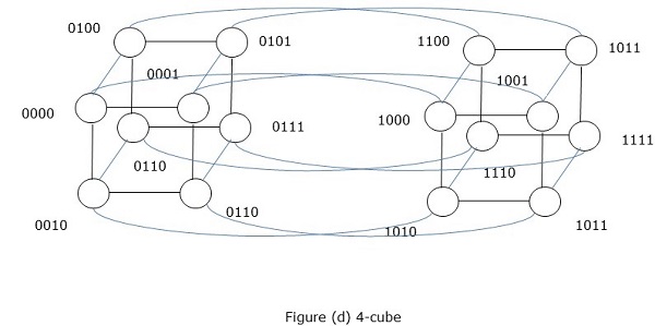
Hypercube Network

Hypercube architecture is helpful for those parallel algorithms where each task has to communicate with other tasks. Hypercube topology can easily embed other topologies such as ring and mesh. It is also known as n-cubes, where n is the number of dimensions. A hypercube can be constructed recursively.

Parallel Algorithm - Design Techniques

Selecting a proper designing technique for a parallel algorithm is the most difficult and important task. Most of the parallel programming problems may have more than one solution. In this chapter, we will discuss the following designing techniques for parallel algorithms −

• Divide and conquer
• Greedy Method
• Dynamic Programming
• Backtracking
• Branch & Bound
• Linear Programming

Divide and Conquer Method

In the divide and conquer approach, the problem is divided into several small sub-problems. Then the sub-problems are solved recursively and combined to get the solution of the original problem.

The divide and conquer approach involves the following steps at each level −

• Divide − The original problem is divided into sub-problems.

• Conquer − The sub-problems are solved recursively.

• Combine − The solutions of the sub-problems are combined together to get the solution of the original problem.

The divide and conquer approach is applied in the following algorithms −

• Binary search
• Quick sort
• Merge sort
• Integer multiplication
• Matrix inversion
• Matrix multiplication

Greedy Method

In greedy algorithm of optimizing solution, the best solution is chosen at any moment. A greedy algorithm is very easy to apply to complex problems. It decides which step will provide the most accurate solution in the next step.

This algorithm is a called greedy because when the optimal solution to the smaller instance is provided, the algorithm does not consider the total program as a whole. Once a solution is considered, the greedy algorithm never considers the same solution again.

A greedy algorithm works recursively creating a group of objects from the smallest possible component parts. Recursion is a procedure to solve a problem in which the solution to a specific problem is dependent on the solution of the smaller instance of that problem.

Dynamic Programming

Dynamic programming is an optimization technique, which divides the problem into smaller sub-problems and after solving each sub-problem, dynamic programming combines all the solutions to get ultimate solution. Unlike divide and conquer method, dynamic programming reuses the solution to the sub-problems many times.

Recursive algorithm for Fibonacci Series is an example of dynamic programming.

Backtracking Algorithm

Backtracking is an optimization technique to solve combinational problems. It is applied to both programmatic and real-life problems. Eight queen problem, Sudoku puzzle and going through a maze are popular examples where backtracking algorithm is used.

In backtracking, we start with a possible solution, which satisfies all the required conditions. Then we move to the next level and if that level does not produce a satisfactory solution, we return one level back and start with a new option.

Branch and Bound

A branch and bound algorithm is an optimization technique to get an optimal solution to the problem. It looks for the best solution for a given problem in the entire space of the solution. The bounds in the function to be optimized are merged with the value of the latest best solution. It allows the algorithm to find parts of the solution space completely.

The purpose of a branch and bound search is to maintain the lowest-cost path to a target. Once a solution is found, it can keep improving the solution. Branch and bound search is implemented in depth-bounded search and depth–first search.

Linear Programming

Linear programming describes a wide class of optimization job where both the optimization criterion and the constraints are linear functions. It is a technique to get the best outcome like maximum profit, shortest path, or lowest cost.

In this programming, we have a set of variables and we have to assign absolute values to them to satisfy a set of linear equations and to maximize or minimize a given linear objective function.

Parallel Algorithm - Matrix Multiplication

A matrix is a set of numerical and non-numerical data arranged in a fixed number of rows and column. Matrix multiplication is an important multiplication design in parallel computation. Here, we will discuss the implementation of matrix multiplication on various communication networks like mesh and hypercube. Mesh and hypercube have higher network connectivity, so they allow faster algorithm than other networks like ring network.

Mesh Network

A topology where a set of nodes form a p-dimensional grid is called a mesh topology. Here, all the edges are parallel to the grid axis and all the adjacent nodes can communicate among themselves.

Total number of nodes = (number of nodes in row) × (number of nodes in column)

A mesh network can be evaluated using the following factors −

• Diameter
• Bisection width

Diameter − In a mesh network, the longest distance between two nodes is its diameter. A p-dimensional mesh network having kP nodes has a diameter of p(k–1).

Bisection width − Bisection width is the minimum number of edges needed to be removed from a network to divide the mesh network into two halves.

Matrix Multiplication Using Mesh Network

We have considered a 2D mesh network SIMD model having wraparound connections. We will design an algorithm to multiply two n × n arrays using n² processors in a particular amount of time.

Matrices A and B have elements a_ij and b_ij respectively. Processing element PE_ij represents a_ij and b_ij. Arrange the matrices A and B in such a way that every processor has a pair of elements to multiply. The elements of matrix A will move in left direction and the elements of matrix B will move in upward direction. These changes in the position of the elements in matrix A and B present each processing element, PE, a new pair of values to multiply.

Steps in Algorithm

• Stagger two matrices.
• Calculate all products, a_ik × b_kj
• Calculate sums when step 2 is complete.

Algorithm

Procedure MatrixMulti

Begin
   for k = 1 to n-1
	
   for all Pij; where i and j ranges from 1 to n
      ifi is greater than k then
         rotate a in left direction
      end if
		
   if j is greater than k then
      rotate b in the upward direction
   end if
	
   for all Pij ; where i and j lies between 1 and n
      compute the product of a and b and store it in c
   for k= 1 to n-1 step 1
   for all Pi;j where i and j ranges from 1 to n
      rotate a in left direction
      rotate b in the upward direction
      c=c+aXb
End

Hypercube Network

A hypercube is an n-dimensional construct where edges are perpendicular among themselves and are of same length. An n-dimensional hypercube is also known as an n-cube or an n-dimensional cube.

Features of Hypercube with 2^k node

• Diameter = k
• Bisection width = 2^k–1
• Number of edges = k

Matrix Multiplication using Hypercube Network

General specification of Hypercube networks −

• Let N = 2^m be the total number of processors. Let the processors be P_0, P₁…..P_N-1.

• Let i and i^b be two integers, 0 < i,i^b < N-1 and its binary representation differ only in position b, 0 < b < k–1.

• Let us consider two n × n matrices, matrix A and matrix B.

• Step 1 − The elements of matrix A and matrix B are assigned to the n³ processors such that the processor in position i, j, k will have a_ji and b_ik.

• Step 2 − All the processor in position (i,j,k) computes the product

  C(i,j,k) = A(i,j,k) × B(i,j,k)

• Step 3 − The sum C(0,j,k) = ΣC(i,j,k) for 0 ≤ i ≤ n-1, where 0 ≤ j, k < n–1.

Block Matrix

Block Matrix or partitioned matrix is a matrix where each element itself represents an individual matrix. These individual sections are known as a block or sub-matrix.

Example

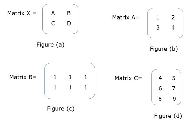
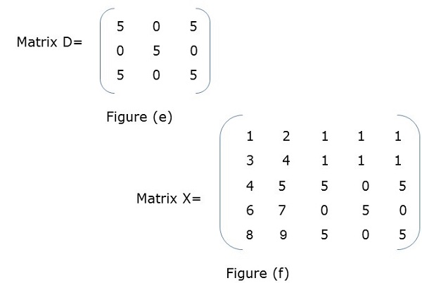
In Figure (a), X is a block matrix where A, B, C, D are matrix themselves. Figure (f) shows the total matrix.

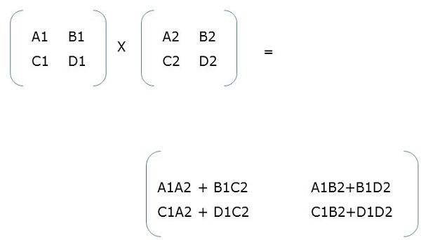
Block Matrix Multiplication

When two block matrices are square matrices, then they are multiplied just the way we perform simple matrix multiplication. For example,

Parallel Algorithm - Sorting

Sorting is a process of arranging elements in a group in a particular order, i.e., ascending order, descending order, alphabetic order, etc. Here we will discuss the following −

• Enumeration Sort
• Odd-Even Transposition Sort
• Parallel Merge Sort
• Hyper Quick Sort

Sorting a list of elements is a very common operation. A sequential sorting algorithm may not be efficient enough when we have to sort a huge volume of data. Therefore, parallel algorithms are used in sorting.

Enumeration Sort

Enumeration sort is a method of arranging all the elements in a list by finding the final position of each element in a sorted list. It is done by comparing each element with all other elements and finding the number of elements having smaller value.

Therefore, for any two elements, a_i and a_j any one of the following cases must be true −

• a_i < a_j
• a_i > a_j
• a_i = a_j

Algorithm

procedure ENUM_SORTING (n)

begin
   for each process P1,j do
      C[j] := 0;
		
   for each process Pi, j do
	
      if (A[i] < A[j]) or A[i] = A[j] and i < j) then
         C[j] := 1;
      else
         C[j] := 0;
			
   for each process P1, j do
      A[C[j]] := A[j];
		
end ENUM_SORTING

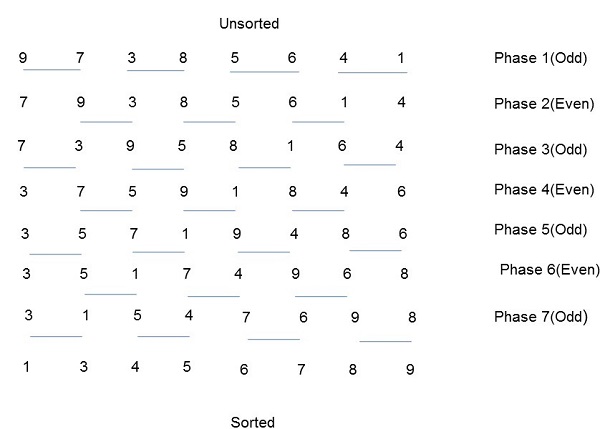
Odd-Even Transposition Sort

Odd-Even Transposition Sort is based on the Bubble Sort technique. It compares two adjacent numbers and switches them, if the first number is greater than the second number to get an ascending order list. The opposite case applies for a descending order series. Odd-Even transposition sort operates in two phases − odd phase and even phase. In both the phases, processes exchange numbers with their adjacent number in the right.

Algorithm

procedure ODD-EVEN_PAR (n) 

begin 
   id := process's label 
	
   for i := 1 to n do 
   begin 
	
      if i is odd and id is odd then 
         compare-exchange_min(id + 1); 
      else 
         compare-exchange_max(id - 1);
			
      if i is even and id is even then 
         compare-exchange_min(id + 1); 
      else 
         compare-exchange_max(id - 1);
			
   end for
	
end ODD-EVEN_PAR

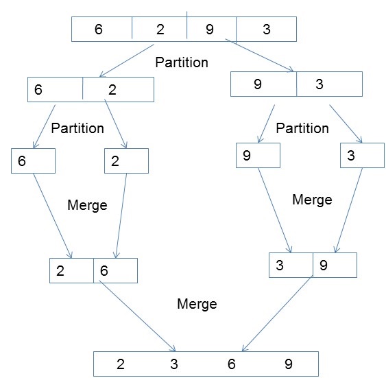
Parallel Merge Sort

Merge sort first divides the unsorted list into smallest possible sub-lists, compares it with the adjacent list, and merges it in a sorted order. It implements parallelism very nicely by following the divide and conquer algorithm.

Algorithm

procedureparallelmergesort(id, n, data, newdata)

begin
   data = sequentialmergesort(data)
	
      for dim = 1 to n
         data = parallelmerge(id, dim, data)
      endfor
		
   newdata = data
end

Hyper Quick Sort

Hyper quick sort is an implementation of quick sort on hypercube. Its steps are as follows −

• Divide the unsorted list among each node.
• Sort each node locally.
• From node 0, broadcast the median value.
• Split each list locally, then exchange the halves across the highest dimension.
• Repeat steps 3 and 4 in parallel until the dimension reaches 0.

Algorithm

procedure HYPERQUICKSORT (B, n)
begin

   id := process’s label;
	
   for i := 1 to d do
      begin
      x := pivot;
      partition B into B1 and B2 such that B1 ≤ x < B2;
      if ith bit is 0 then
		
      begin
         send B2 to the process along the ith communication link;
         C := subsequence received along the ith communication link;
         B := B1 U C;
      endif
      
      else
         send B1 to the process along the ith communication link;
         C := subsequence received along the ith communication link;
         B := B2 U C;
         end else
      end for
		
   sort B using sequential quicksort;
	
end HYPERQUICKSORT

Parallel Search Algorithm

Searching is one of the fundamental operations in computer science. It is used in all applications where we need to find if an element is in the given list or not. In this chapter, we will discuss the following search algorithms −

• Divide and Conquer
• Depth-First Search
• Breadth-First Search
• Best-First Search

Divide and Conquer

In divide and conquer approach, the problem is divided into several small sub-problems. Then the sub-problems are solved recursively and combined to get the solution of the original problem.

The divide and conquer approach involves the following steps at each level −

• Divide − The original problem is divided into sub-problems.

• Conquer − The sub-problems are solved recursively.

• Combine − The solutions of the sub-problems are combined to get the solution of the original problem.

Binary search is an example of divide and conquer algorithm.

Pseudocode

Binarysearch(a, b, low, high)

if low < high then
   return NOT FOUND
else
   mid ← (low+high) / 2
   if b = key(mid) then
      return key(mid)
   else if b < key(mid) then
      return BinarySearch(a, b, low, mid−1)
   else
   
      return BinarySearch(a, b, mid+1, high)

Depth-First Search

Depth-First Search (or DFS) is an algorithm for searching a tree or an undirected graph data structure. Here, the concept is to start from the starting node known as the root and traverse as far as possible in the same branch. If we get a node with no successor node, we return and continue with the vertex, which is yet to be visited.

Steps of Depth-First Search

• Consider a node (root) that is not visited previously and mark it visited.

• Visit the first adjacent successor node and mark it visited.

• If all the successors nodes of the considered node are already visited or it doesn’t have any more successor node, return to its parent node.

Pseudocode

Let v be the vertex where the search starts in Graph G.

DFS(G,v)

   Stack S := {};
	
   for each vertex u, set visited[u] := false;
   push S, v;
   while (S is not empty) do
     u := pop S;
	  
      if (not visited[u]) then
         visited[u] := true;
         for each unvisited neighbour w of u
            push S, w;
      end if
		
   end while
   
END DFS()

Breadth-First Search

Breadth-First Search (or BFS) is an algorithm for searching a tree or an undirected graph data structure. Here, we start with a node and then visit all the adjacent nodes in the same level and then move to the adjacent successor node in the next level. This is also known as level-by-level search.

Steps of Breadth-First Search

• Start with the root node, mark it visited.
• As the root node has no node in the same level, go to the next level.
• Visit all adjacent nodes and mark them visited.
• Go to the next level and visit all the unvisited adjacent nodes.
• Continue this process until all the nodes are visited.

Pseudocode

Let v be the vertex where the search starts in Graph G.

BFS(G,v)

   Queue Q := {};
	
   for each vertex u, set visited[u] := false;
   insert Q, v;
   while (Q is not empty) do
      u := delete Q;
		
      if (not visited[u]) then
         visited[u] := true;
         for each unvisited neighbor w of u
            insert Q, w;
      end if
		
   end while
   
END BFS()

Best-First Search

Best-First Search is an algorithm that traverses a graph to reach a target in the shortest possible path. Unlike BFS and DFS, Best-First Search follows an evaluation function to determine which node is the most appropriate to traverse next.

Steps of Best-First Search

• Start with the root node, mark it visited.
• Find the next appropriate node and mark it visited.
• Go to the next level and find the appropriate node and mark it visited.
• Continue this process until the target is reached.

Pseudocode

BFS( m )

   Insert( m.StartNode )
   Until PriorityQueue is empty
      c ← PriorityQueue.DeleteMin
      If c is the goal
      Exit
   Else
   
      Foreach neighbor n of c
         If n "Unvisited"
            Mark n "Visited"
            Insert( n )
      Mark c "Examined"
      
End procedure

Graph Algorithm

A graph is an abstract notation used to represent the connection between pairs of objects. A graph consists of −

• Vertices − Interconnected objects in a graph are called vertices. Vertices are also known as nodes.

• Edges − Edges are the links that connect the vertices.

There are two types of graphs −

• Directed graph − In a directed graph, edges have direction, i.e., edges go from one vertex to another.

• Undirected graph − In an undirected graph, edges have no direction.

Graph Coloring

Graph coloring is a method to assign colors to the vertices of a graph so that no two adjacent vertices have the same color. Some graph coloring problems are −

• Vertex coloring − A way of coloring the vertices of a graph so that no two adjacent vertices share the same color.

• Edge Coloring − It is the method of assigning a color to each edge so that no two adjacent edges have the same color.

• Face coloring − It assigns a color to each face or region of a planar graph so that no two faces that share a common boundary have the same color.

Chromatic Number

Chromatic number is the minimum number of colors required to color a graph. For example, the chromatic number of the following graph is 3.

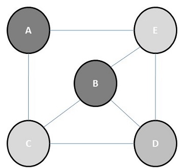
The concept of graph coloring is applied in preparing timetables, mobile radio frequency assignment, Suduku, register allocation, and coloring of maps.

Steps for graph coloring

• Set the initial value of each processor in the n-dimensional array to 1.

• Now to assign a particular color to a vertex, determine whether that color is already assigned to the adjacent vertices or not.

• If a processor detects same color in the adjacent vertices, it sets its value in the array to 0.

• After making n² comparisons, if any element of the array is 1, then it is a valid coloring.

Pseudocode for graph coloring

begin

   create the processors P(i0,i1,...in-1) where 0_iv < m, 0 _ v < n
   status[i0,..in-1] = 1
	
   for j varies from 0 to n-1 do
      begin
		
         for k varies from 0 to n-1 do
         begin
            if aj,k=1 and ij=ikthen
            status[i0,..in-1] =0
         end
			
      end
      ok = ΣStatus
		
   if ok > 0, then display valid coloring exists
   else
      display invalid coloring
      
end

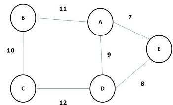
Minimal Spanning Tree

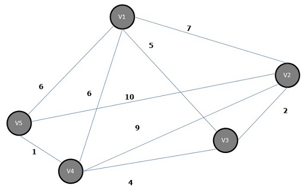
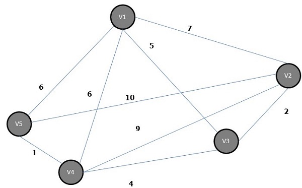
A spanning tree whose sum of weight (or length) of all its edges is less than all other possible spanning tree of graph G is known as a minimal spanning tree or minimum cost spanning tree. The following figure shows a weighted connected graph.

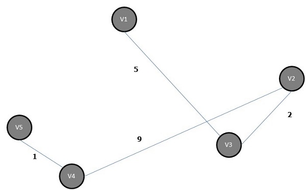
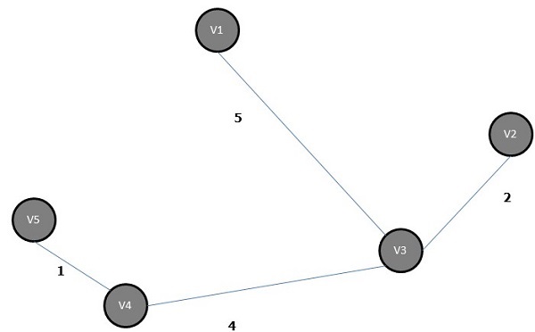
Some possible spanning trees of the above graph are shown below −

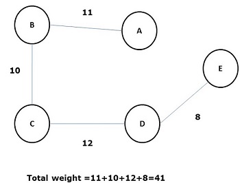
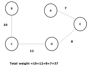
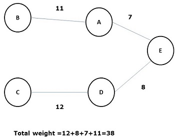
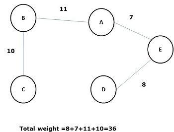
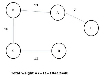
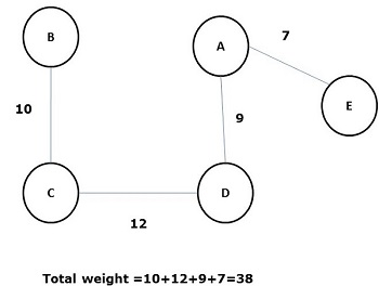
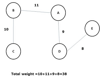
Among all the above spanning trees, figure (d) is the minimum spanning tree. The concept of minimum cost spanning tree is applied in travelling salesman problem, designing electronic circuits, Designing efficient networks, and designing efficient routing algorithms.

To implement the minimum cost-spanning tree, the following two methods are used −

• Prim’s Algorithm
• Kruskal’s Algorithm

Prim's Algorithm

Prim’s algorithm is a greedy algorithm, which helps us find the minimum spanning tree for a weighted undirected graph. It selects a vertex first and finds an edge with the lowest weight incident on that vertex.

Steps of Prim’s Algorithm

• Select any vertex, say v₁ of Graph G.

• Select an edge, say e₁ of G such that e₁ = v₁ v₂ and v₁ ≠ v₂ and e₁ has minimum weight among the edges incident on v₁ in graph G.

• Now, following step 2, select the minimum weighted edge incident on v₂.

• Continue this till n–1 edges have been chosen. Here n is the number of vertices.

The minimum spanning tree is −

Kruskal's Algorithm

Kruskal’s algorithm is a greedy algorithm, which helps us find the minimum spanning tree for a connected weighted graph, adding increasing cost arcs at each step. It is a minimum-spanning-tree algorithm that finds an edge of the least possible weight that connects any two trees in the forest.

Steps of Kruskal’s Algorithm

• Select an edge of minimum weight; say e₁ of Graph G and e₁ is not a loop.

• Select the next minimum weighted edge connected to e₁.

• Continue this till n–1 edges have been chosen. Here n is the number of vertices.

The minimum spanning tree of the above graph is −

Shortest Path Algorithm

Shortest Path algorithm is a method of finding the least cost path from the source node(S) to the destination node (D). Here, we will discuss Moore’s algorithm, also known as Breadth First Search Algorithm.

Moore’s algorithm

• Label the source vertex, S and label it i and set i=0.

• Find all unlabeled vertices adjacent to the vertex labeled i. If no vertices are connected to the vertex, S, then vertex, D, is not connected to S. If there are vertices connected to S, label them i+1.

• If D is labeled, then go to step 4, else go to step 2 to increase i=i+1.

• Stop after the length of the shortest path is found.