
Article Categories
- All Categories
-
 Data Structure
-
 Networking
-
 RDBMS
RDBMS
-
 Operating System
-
 Java
Java
-
 MS Excel
-
 iOS
iOS
-
 HTML
HTML
-
 CSS
CSS
-
 Android
-
 Python
-
 C Programming
-
 C++
C++
-
 C#
C#
-
 MongoDB
-
 MySQL
MySQL
-
 Javascript
-
 PHP
PHP
-
 Economics & Finance
How to sort data by text, date, number or color in Excel
Excel has the capability to automatically include related data into a range, provided that there are no empty rows or columns inside the area that has been specified. It is ok to leave empty rows and columns between groups of related data. Excel will then examine the data area to see whether it contains any field names, and if it does, it will remove rows containing those names from the set of records that will be sorted.
Filtering and sorting are two of the most useful functions that can be found in Microsoft Excel. In the field of data analysis, they are utilized extensively for the purposes of organizing, arranging, and subsetting your data based on a variety of variables.
Excel's numerous built-in choices have made data sorting a breeze, making it one of the program's more user-friendly features. You have the option to sort your data in a variety of ways, including alphabetically, according to the value in the cells, or by the color of the cells and font.
In this tutorial, you are going to learn how to sort data by text, date, number or color.
Sort Data by Text
You can follow the procedures given below to sort a range of data based on texts, in ascending or descending order.
Step 1
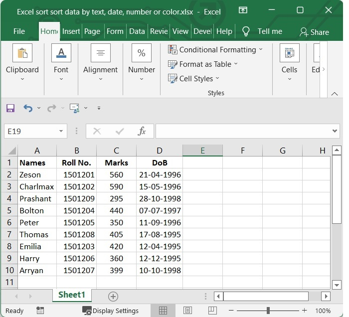
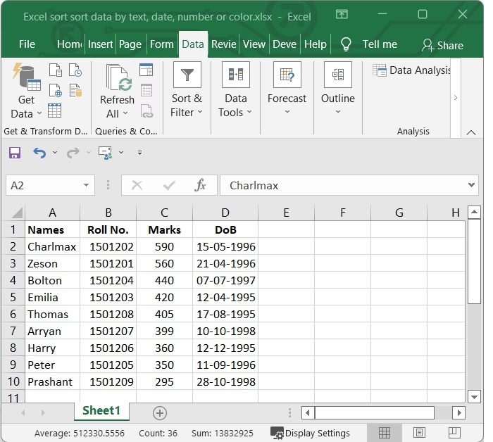
In our example, we have name of some students with roll number and marks in an Excel sheet. See the screenshot below.
Step 2
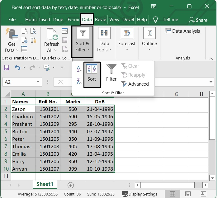
After that make a selection of the data range that you want to sort. Then go to the Sort menu of Data tab.
Step 3
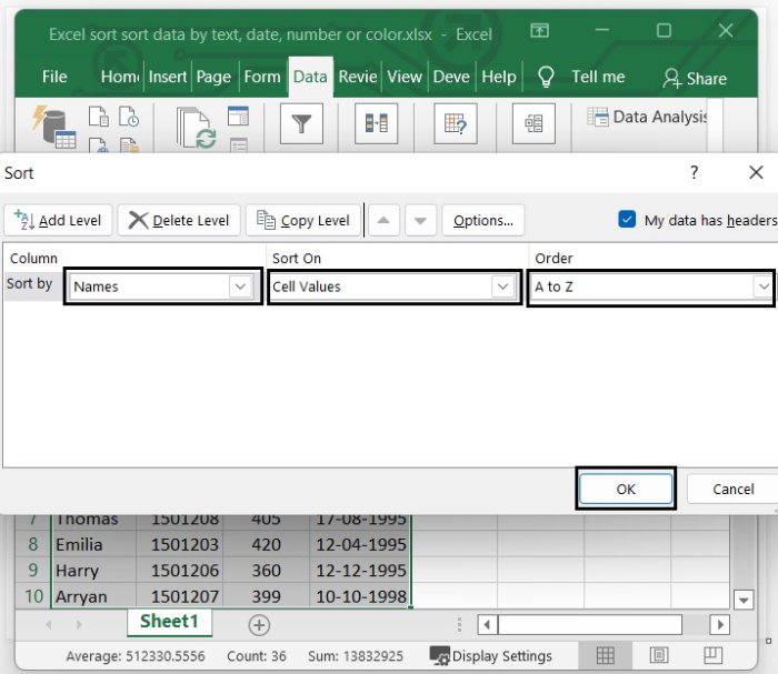
In the Sort dialog box, Choose the column whose name you would want to sort the data by in the section labelled Column. Then choose the option Cell Values to sort by in the section titled Sort On. Specify the order of the sort in the area labelled Order. Then click on OK.
In our case, we have sorted the sheet according to name and the order is A-Z.
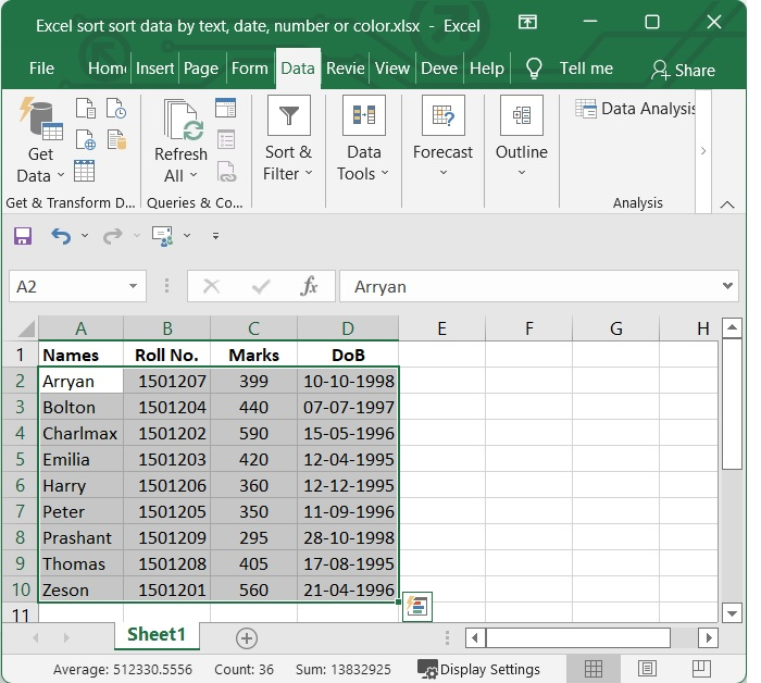
After sorting, our Excel sheet will look like as the image given below.
Sort Data by Numbers
Step 1
In the above example, let?s suppose we want to sort the data by marks scored by the students. Follow the steps given below.
Select the range of the data that you wish to be sorted before continuing. After that, select the Data tab in Excel and go to the Sort menu. Take a look at the following screenshot.

Step 2
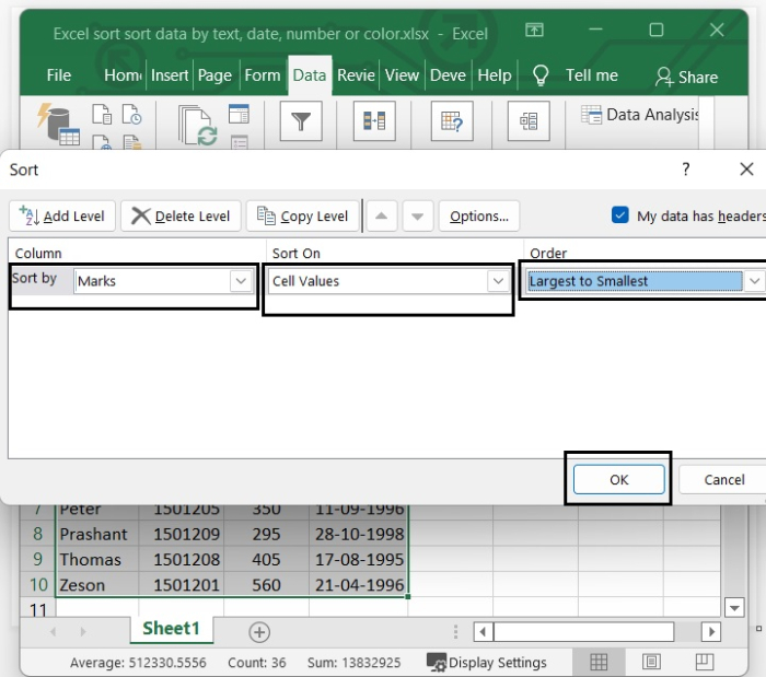
Choose the column name in which the numbers are written in the part of the Sort dialogue box labelled Column. This will cause the data to be sorted in the desired order. Then, under the section that is titled Column, select the option that is labelled Cell Values to sort by. Indicate the order in which the sort should be performed in the box labelled Order. The next step is to click the OK button.
In our example, we have sorted the sheet in numerical order thorough the column named as "Marks" and the order of sorting is largest to smallest. Take a look at the screenshot that is provided below.
After sorting, our Excel sheet will look like as the image given below.
Sort Data by Date
Let?s suppose in the above excel sheet, there is Date of Birth column and we want to sort the data by Date. Follow the below given steps.
Step 1
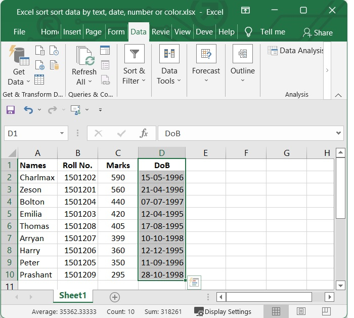
Our Excel sheet contains the data as shown in the following screenshot.
Step 2
After that, select the data range that you wish to sort. After that, select the Data tab in Excel and go to the Sort menu. Take a look at the screenshot that is given below.

Step 3
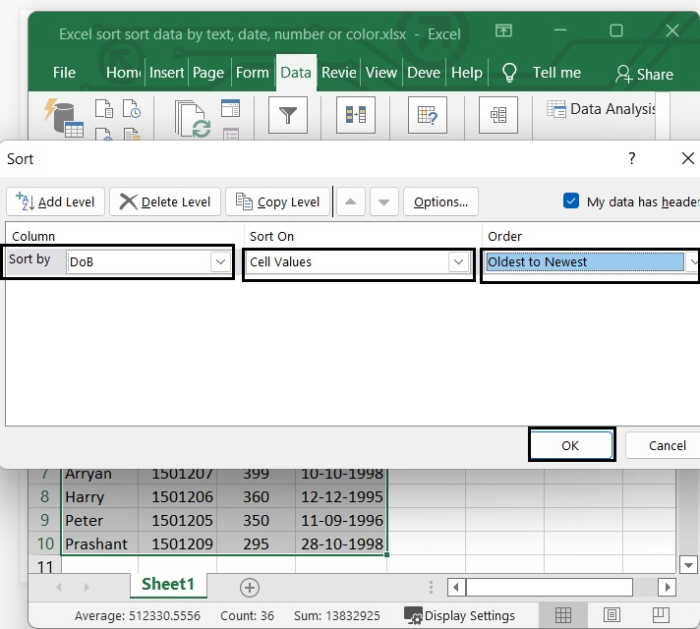
In the portion of the Sort dialogue box that is labelled Column, you will need to select the column name in which the DATES are written. The data will be sorted into the desired order as a result of this action. Then, under the section that is titled Sort On, choose the option that is labelled Cell Values to sort by. This will allow you to sort the data according to the cell values.
In the box labelled "Order," select Newest to Oldest or Oldest to Newest to sort the items in the correct order. Then click OK button.
In our example, the column name is DoB that is selected and the order is Oldest to Newest.
After sorting, the sheet will look like the one given below ?

Sort Data by Color
If you want to sort the data range depending on the color of the cells, the color of the font, or an icon for conditional formatting, you may do this work easily by using the Sort function.
Step 1
Suppose in our Excel, we have a data range which has some coloured cells, as shown in the screenshot below.
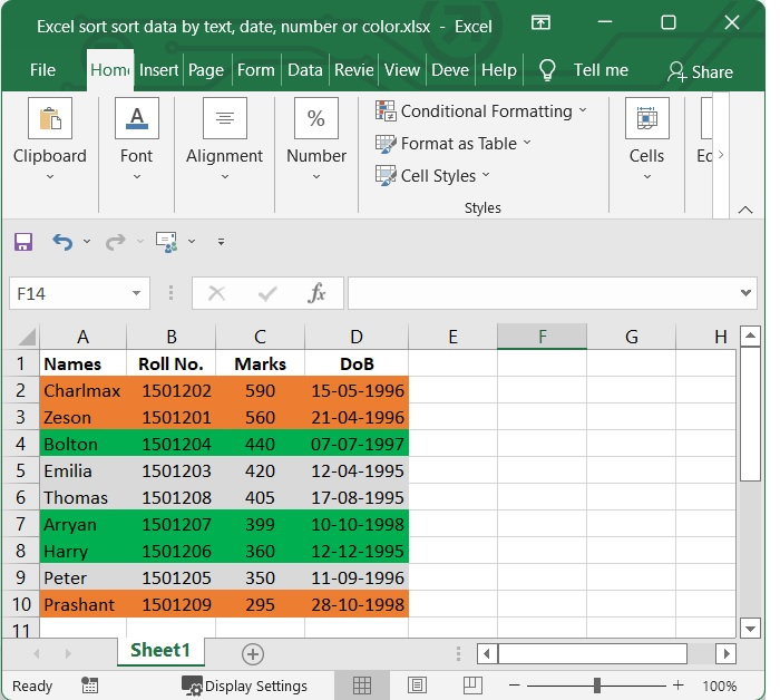
We need to rearrange the cells as per the colour. For example, orange colour on the top then grey colour and then green colour. Follow the steps given below.
Step 2
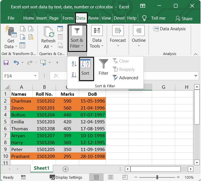
Select the range of the data that you wish to be sorted before continuing. After that, select the Data tab in Excel and go to the Sort menu.
Step 3
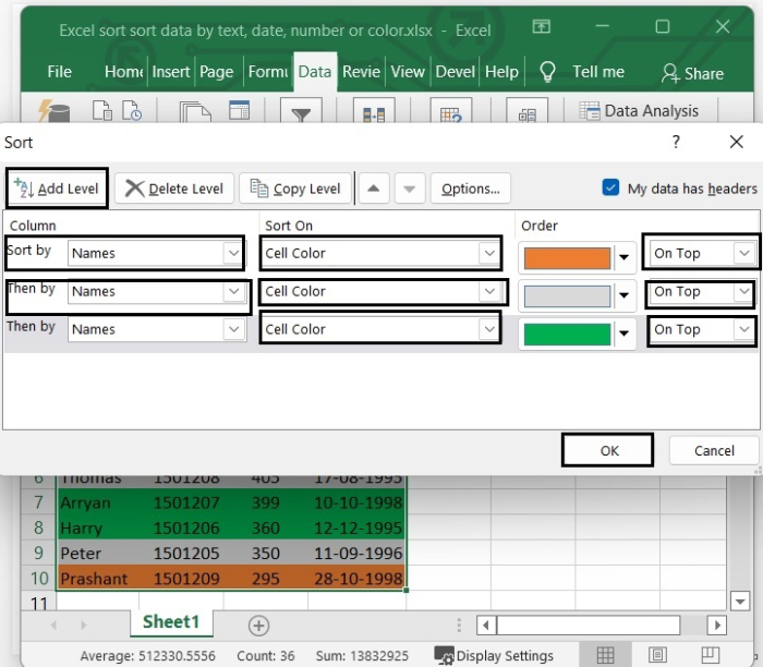
In the "Column" section, choose "Name" or one of the other columns where the coloured cells are. Then choose the Cell Color option under the "Sort on" section. Then, choose the colour cell you want to be on top or bottom in the Order section.
Then, click the "Add Level" button to add another level and repeat the above setting to set the colours for the second and any other rule levels. See the below given image.
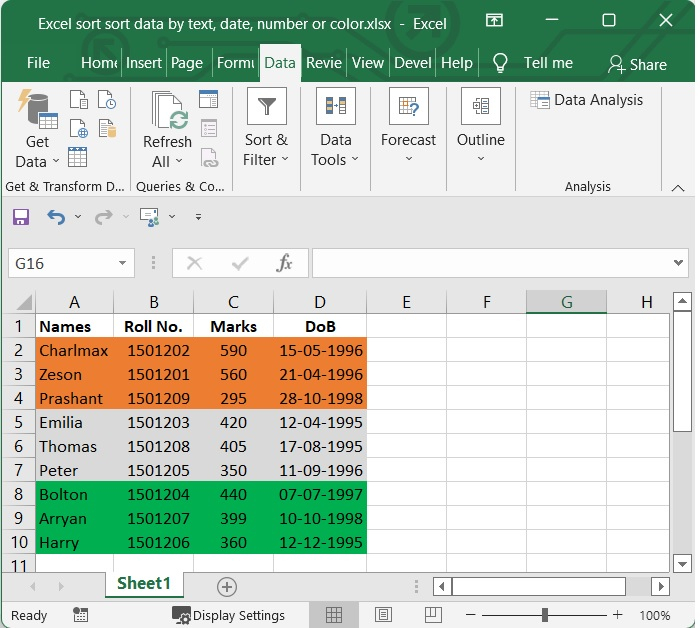
After setting the colour, click OK. After arranging the colour, the Excel sheet will look like as given below.

517 Views
