How to Preserve Grid Lines While Filling Color in Excel?

Let us assume that we are working in an excel sheet. Now there are chances that we need to fill color in the excel sheet to highlight the data or we want to differentiate the data. Filling colors in the excel sheet can prove to be very helpful. Now there is one problem that occurs, and that problem is that when we fill the color in excel sheet, the grid lines of which the whole spreadsheet is composed of, disappears. Grid lines are simple horizontal and vertical lines which make up the whole excel spreadsheet. It is the gridlines that give definition to the spreadsheet. So read this tutorial to learn how to preserve gridlines while filling color in excel.

Data Example

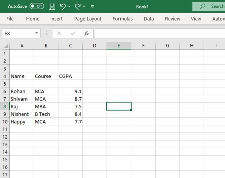
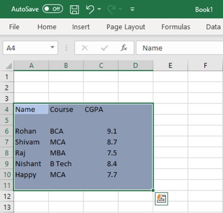
Now to illustrate this problem we will take an example of a simple dataset. The dataset comprises a list of some students with their course and obtained cgpa.

As we can see in this example, the gridlines are visible by default.

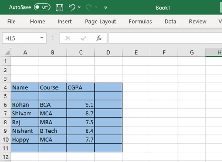
Now in this example we have applied a fill color feature in the cell range A4:D11 and we can see that in that range area the grid lines have disappeared. This is the problem that we have to deal with.

Methods to Preserve Gridlines After using Color in Excel

Excel provides many different functionalities that we can use to perform various operations. So in case of this problem, there are basically 3 methods by which we can preserve gridlines after using color in excel.

Using Borders Drop−Down Feature

This feature is one of the simplest features that we use to preserve gridlines after using color in excel. It’s just a four step process. The steps are as follows :

• First, select the area where we want to preserve our gridlines. In our example it is A4:D11.

• After that go to Home. Then in the font section, the Borders drop down menu is there.

• Click on that Borders Drop−Down icon.

• There are many options visible. Select the option All Borders.

• Now finally we will see that the gridlines are again visible in the desired area.

In the screenshot below we can clearly see that by applying the above process the grid lines are now visible.

Using Custom Cell Style Option to Preserve Gridlines

In this method, we are actually formatting the cell style to preserve the gridlines. In this we will not be using the fill color option, instead we will be formatting the cell style to fill the color and at the same time preserving the gridlines.

Now in the above screenshot we can see that we have not used any fill in color option. Now to perform this method, the steps are as follows :

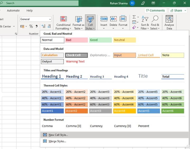
• Select Home. After that select Styles −> Cell Styles −> New Cell Style.

• Now after clicking on New Cell Style, Style dialog box will open.

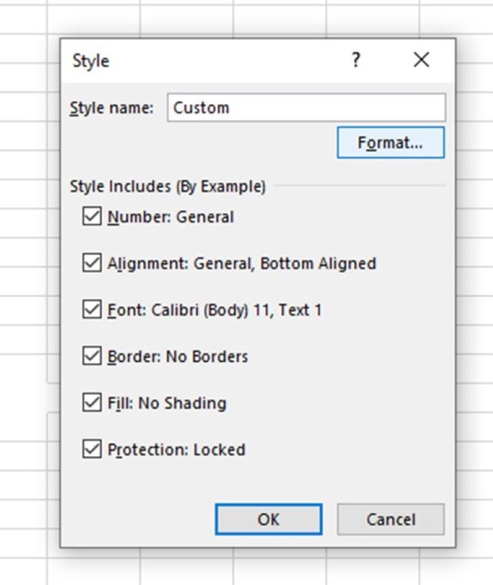
• Now in the Style name, type any custom style name that you want. Here we are choosing the name custom.

• After typing the name custom, click on the Format button.

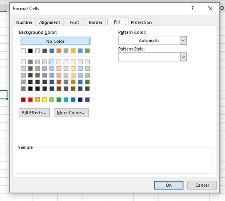
• Now we will see that a new dialog box has emerged.

• So, in the Fill tab, select any color of your choice. Here we are selecting the blue color.

• Now go to the Border tab. Here we select the gray color. We are selecting the gray color in order to match the color with the gridlines.

• At last, click the OK button.

• Now we can clearly see that in the screenshot below the color and the gridlines are clearly visible.

Using Format Cell Feature to Preserve Gridlines

This is also a wonderful feature that excel has provided which we can use to preserve our gridlines while filling color in excel. This feature is used after using the Fill color feature. To use this method follow the steps below :

• Firstly select the coloured range on which we want to preserve our gridlines. In our case it is A4:D11.

• Now after that press ctrl + 1. This is the shortcut to open the Format cell dialog box.

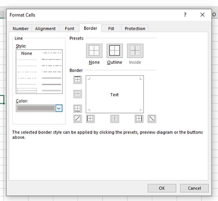
• After pressing the shortcut, the Format Cell dialog box will open.

• Now select the Border tab. Here we select the gray color. We are selecting the gray color in order to match the color with the gridlines.

• After this in the Presets option, select the Outline and Inside option.

• At last, click the OK button.

• Now we can clearly see that in the screenshot below the color and the gridlines are clearly visible.

Conclusion

So in this tutorial we have learnt how to preserve gridlines while filling color in excel. Here we have learnt 3 methods which are as follows:

• Using Borders Drop−Down feature

• Using Custom Cell style option to preserve gridlines

• Using Format Cell feature to preserve gridlines

These 3 methods are very simple to implement. So use them and we will be happy if you can share with us some new methods by which we can preserve our gridlines while filling color in excel. You can drop down your suggestions, queries, any new idea in the comment section below.