How to Preserve Formatting After Refreshing Pivot Table?

With the help of pivot tables, you can swiftly analyse and summarise massive amounts of data. Maintaining the formatting of pivot tables while updating them with new data is a problem that many users run across. Have you ever worked hard to format a pivot table to perfection only to have it all vanish the moment you hit the refresh button? You're not alone, so don't worry! In this lesson, we'll show you how to take the necessary precautions to make sure that your pivot table's formatting holds up even after the underlying data has been refreshed.

So let's get started and learn how to make the formatting of your pivot table resistant to modifications. By the time you finish this article, you'll be confidently able to update your pivot tables in Excel without sacrificing the desired formatting. Let's get going!

Preserve Formatting After Refreshing Pivot Table

Here we will format the pivot table to complete the task. So let us see a simple process to know how you can preserve formatting after refreshing a pivot table in Excel.

Step 1

Consider an Excel sheet where you have a pivot table.

First, right-click on any pivot table cell and select the PivotTable option.

Right Click > PivotTable Option.

Step 2

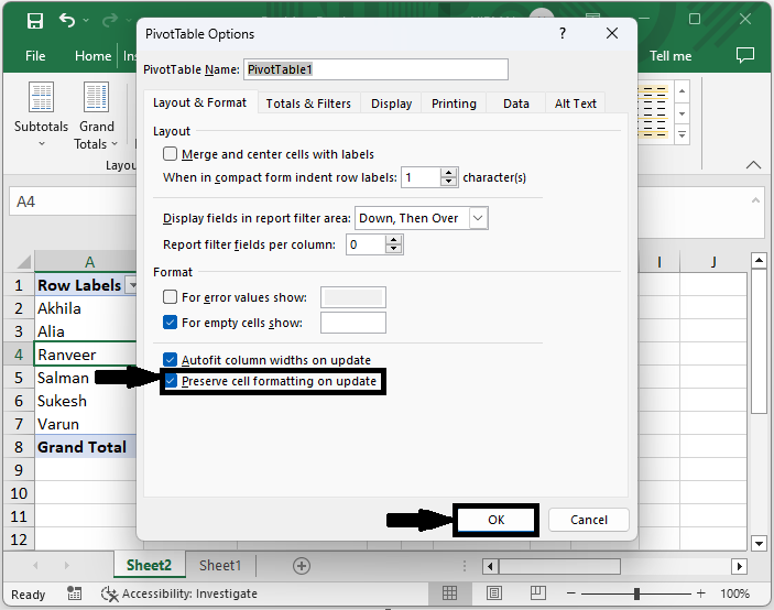
Then click on Layout and Format, then click the box named Preserve cell formatting on Update under Format.

Layout and Format > Check Box.

Step 3

Then click OK to complete the task. From now on, when you refresh the pivot table, the format will be preserved.

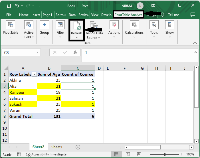
This is how you can preserve formatting after refreshing a pivot table in Excel.

Conclusion

In this tutorial, we have used a simple example to demonstrate how you can preserve formatting after refreshing a pivot table in Excel to highlight a particular set of data.

Pradeep Kumar

e

Updated on: 07-Sep-2023

500 Views

Kickstart Your Career

Get certified by completing the course

Get Started