How to merge and combine rows without losing data in Excel?

In the article, the users are going to merge and combine the rows without losing any data in Microsoft Excel. There are numerous types of structures within the Excel sheet including formula, Combine rows & columns, and formulas that will merge and combine the rows according to the need. The users can use the Combine rows & columns from the Ku-tools tab to combine the values. This method may be completed utilizing an easy way within Microsoft Excel by using the formula and Combining rows & columns.

Let’s explore the articles with few examples

Example 1: By using user defined formula

Step 1

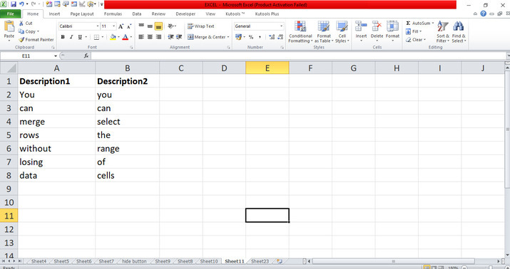
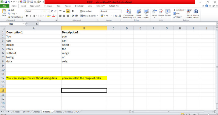
Deliberate the Excel worksheet. First, open the Excel sheet and create the data one by one from cell A1 to B8 in any cell according to the need to merge the data as shown below.

Step 2

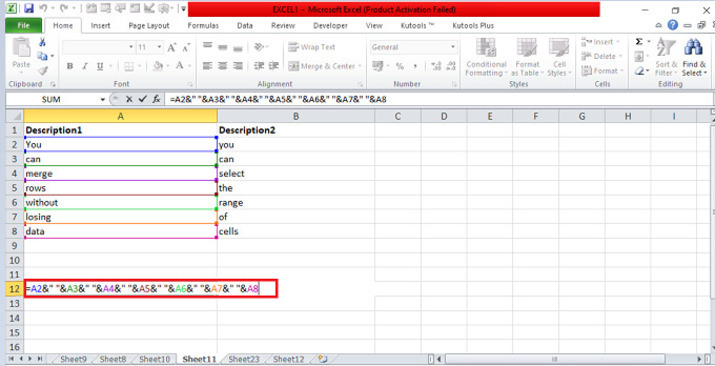
In the sheet, they have to concatenate the multiple rows that are included. To concatenate the data, use the formula. Place the cursor in the cell A12 and enter the formula =A2&" "&A3&" "&A4&" "&A5&" "&A6&" "&A7&" "&A8 and press Enter tab that will concatenate or merge the rows for the row A as shown below.

Step 3

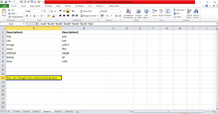
In the sheet, after merging the rows, we have to highlight the cell. Open the Fill Color which is included on Home tab. Place the cursor on it and choose the yellow color to highlight the merged cell A12 as shown below.

Step 4

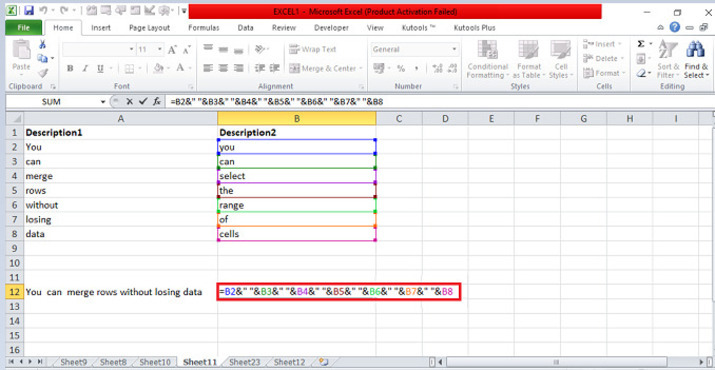
In the sheet, they have to concatenate the multiple rows that are included. To concatenate the data, use the formula. Place the cursor in the cell B12 and enter the formula =B2&" "&B3&" "&B4&" "&B5&" "&B6&" "&B7&" "&B8 and press Enter tab that will concatenate or merge the rows for the row B as shown below.

Step 5

In the sheet, after merging the rows, we have to highlight the cell. Open the Fill Color which is included on Home tab. Place the cursor on it and choose the yellow color to highlight the merged cell B12 as shown below.

Example 2: By using Kutools

Step 1

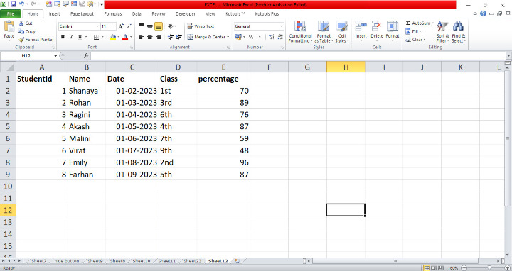
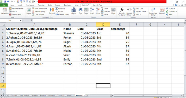
Deliberate the Excel worksheet. First, open the Excel sheet and create the data one by one from cell A1 to B8 in any cell according to the need to merge the data as shown below.

Step 2

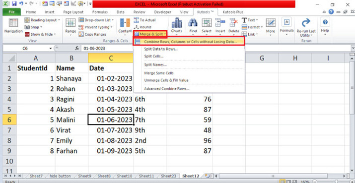
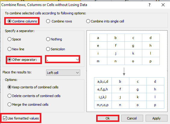
Place the cursor in the ribbon. In the ribbon, there are many tabs included in the top corner. Place the cursor in the Ku-tools tab and click on the tab that has many options included. On the Ku-tools tab, place the cursor and click on the Merge & Split tab which has a drop-down menu on the Ranges & Cells group. Click on the menu and select Combine Rows, Columns, or Cells without losing the data tab that will open the dialog box as shown below.

Step 3

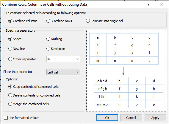
In the dialog box, enable the option Combine columns and place the cursor in the Other Separator option then enable it. Place the cursor in the drop-box of the separator and enter the symbol comma in the box. Then place the cursor and enable the option Use Formatted Values in the bottom area then click on the ok button as shown below.

Step 4

In the sheet, it will combine the columns automatically in row A as shown below.

The users utilized the easy instances to display how they merge and combine rows without losing any data differently by using the formula tab and Ku-tools tab. The users used the necessary tabs which are included in the ribbon. They have to practice the essential options from the ribbon and modify the data according to the need.