How to format the cell value red if negative and green if positive in Excel?

Cell formatting is wonderful feature of Microsoft excel where cell value or text font size, type, color, background color may be formatted based on different criteria. In this, methods for format cell value font color based on a given condition have discussed. Here, a default color of cell value is changed in red color when value is negative and green color when cell value is positive. Further section presents, methods of cell value color formatting with suitable examples.

Format cell value red if it is negative or green when it is positive in Excel

To format cell value color, two methods may be used. Both methods listed below and present their working individually in details.

• Method-1: Using conditional formatting

• Method-2: Using select specific cells

Method-1: Using Conditional Formatting

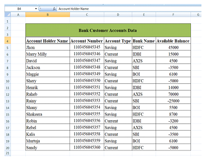
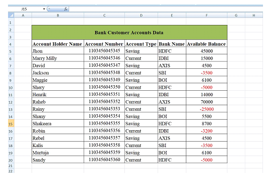
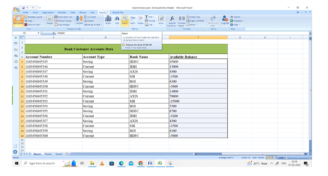
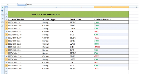
With the help of conditional formatting feature of excel, we can format cell value color based on given constraints. To demonstrate this approach, we have considered sample data of bank customer accounts which contains Customer Name, Account Number, Account Type, Bank Name, Available Balance fields. Here, Account balance of customer may be zero, positive or negative number. Therefore, to filler out customers those balances is negative via format respective cell in red color and those balances are non-positive and greater than zero via format cell in green color then conditional formatting approach is employed. Data of customer is show in below sheet.

Using Conditional Formatting: To format cell value color red if value is negative and green if value is positive, conditional formatting works in following steps.

Step 1

Select the required cells ranges F5:F20 on which require applying format.

Step 2

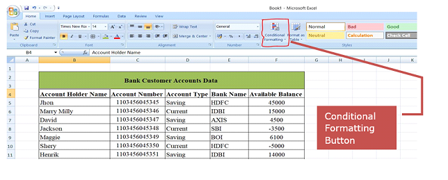
Go to Home tab of excel workbook and click on Conditional Formatting button that shows in below figure.

Step 3

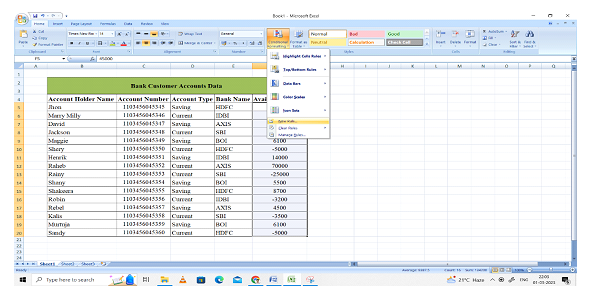
Click on New Rule on conditional formatting menu. Then new formatting rule window is opened.

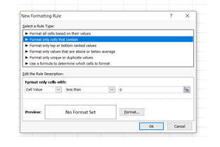
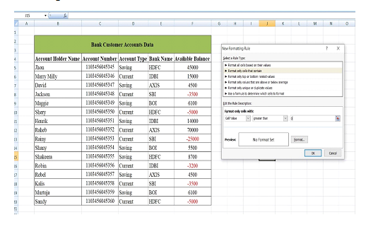
Step 4

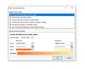
Select the “Format only cells that contain” option in the new rule window and then select cell value, less than 0 options in the format cell with only window as shown in below image.

Step 5

Click on the Format button of New Formatting Rule window then Format Cells window is opened.

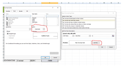
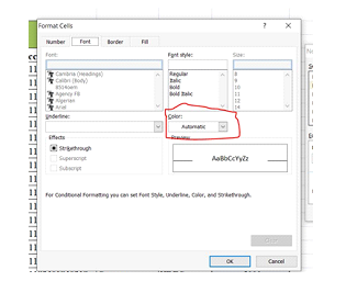
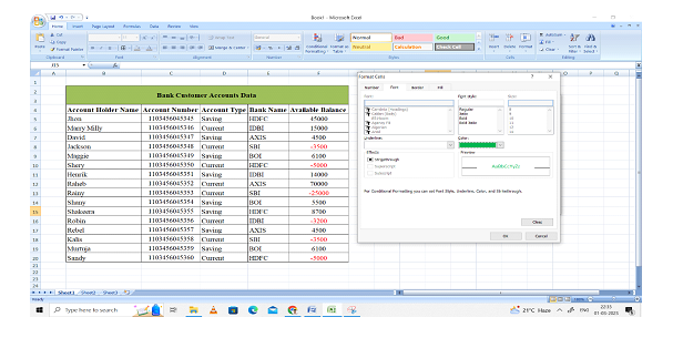
Step 6

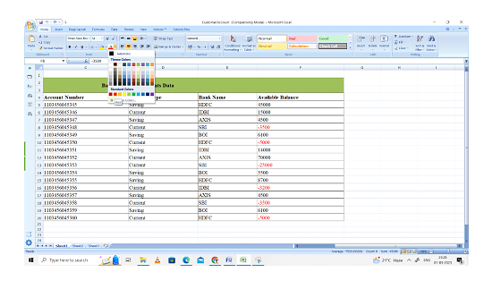
Click Font tab of Format Cells dialog box and click on Color option as shown below:

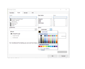
Step 7

Font color panel is opened. Choose color of font as red then click on OK button of format cells window then again click on OK button of New Formatting Rule window.

Step 8

After the step-7, the font color of selected cells becomes red that contains the negative. The results are shown in below figure.

Similarly, all above steps are followed for format cell value with color if value is positive or greater than 0. For this, we again create new rule using same steps and define cell value, greater than 0 option and select green font color of cell value as shown in below figures.

Approach 2: Using Select Specific Cell

Another approach to format cell value is select specific cell. This approach works in following steps.

Step 1

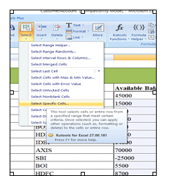
Select cells on which format will apply. Click Select option of Kutools extension of excel. It shows below.

Step 2

Once clicked on select option of Kutools tab. It shows menus of various option. Then click on Select Specific Cells option as shown in below images.

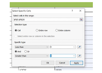
Step 3

After this, Select Specific Cells window is opened. In this window, we select cell option as selection type and select “less than” 0 and “greater than” 0 as specific type option. It is shows below.

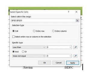
Step 4

Click on Apply button of Select Specific Cells window. In this window, we select cell option as Selection type and select “Less than” 0 and “does not equal” to 0 as specific type option then cell those value is negative selected as shown below:

Step 5

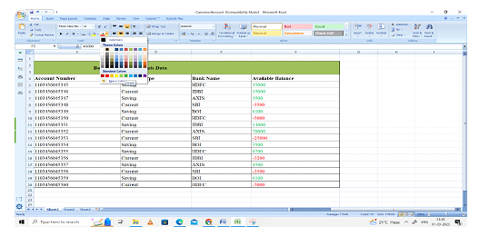
Go to the Home tab and click on Font color option. Select Red color then all selected cell value color becomes red which is negative as illustrated in below image.

Similarly, all above steps are followed for format cell value with color green if value is positive or greater than 0. For this, we again create select cell option as selection type and select “greater than” 0 and “not equal to” 0 as specific type option then cells selected those value are positive as shown in below image:

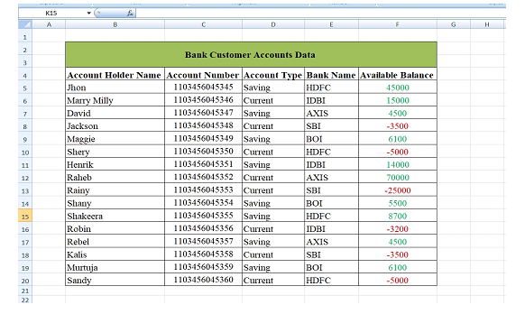
At last, cell value is formatted in red and green font color according to negative and positive available balance of customer account as highlighted in below image:

Conclusion

This article was presented conditional formatting of cell value with color red if it is negative and color green if value is positive. For demonstration of this, a bank customer account data in excel sheet was considered as an example. In this data, Available balance of customer may be positive and negative. We have applied conditional formatting on the available balance field of customer data.