How to find the largest negative value (less than 0) in Excel?

Sometimes the scenario may come how to find the most negative value possible in your Excel spreadsheet. Imagine that instead of positive numbers there are hundreds of thousands of lines filled with negative numbers. The formula which you will learn in this tutorial will prove useful in the circumstances like this.

The formula uses a few standard functions in order to locate the cell in an Excel spreadsheet that contains the most significant negative number. The IF function and the MAX function are both incorporated into this formula.

Let’s see step by step with an example.

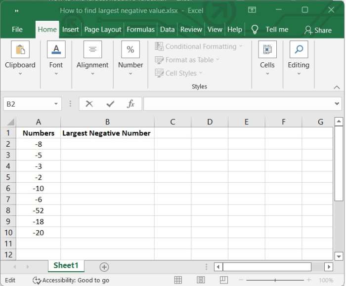
Step 1

In our example we have some negative numbers and positive numbers in our Excel sheet. Refer the following image −

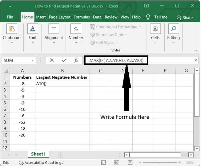
Step 2

Select a blank cell B2 and type the following formula in the formula bar.

=MAX(IF( A2:A10<0, A2:A10))

The purpose of the IF function in this formula is to filter the data in such a way that the MAX function receives only those values from the filtered set that satisfy the conditions that have been specified.

• In Microsoft Excel, the beginning of any function is denoted by the equal sign, which is written as =.

• Our IF function is denoted by the notation IF(). To ensure that the function is successfully executed, we will need to place the logical expression, value if true, and value if false inside of the brackets.

• Logical expression is the condition for which we are looking for an answer as True or False

• If the logical expression is evaluated as true, the value that is returned is referred as value if true.

• If the logical expression is found to be false, the value that is returned is referred as value if false.

When you need to determine which numeric dataset contains the highest number, the MAX function can be quite helpful. Within the context of this formula, the purpose of the MAX function is to return the filtered data point that contains the biggest negative value.

See the following image to get a clear idea.

Step 3

After entering the formula, press Shift + Ctrl+ Enter to get calculated the formula.

Then the largest negative number will be written in B2 cell. See the following image −

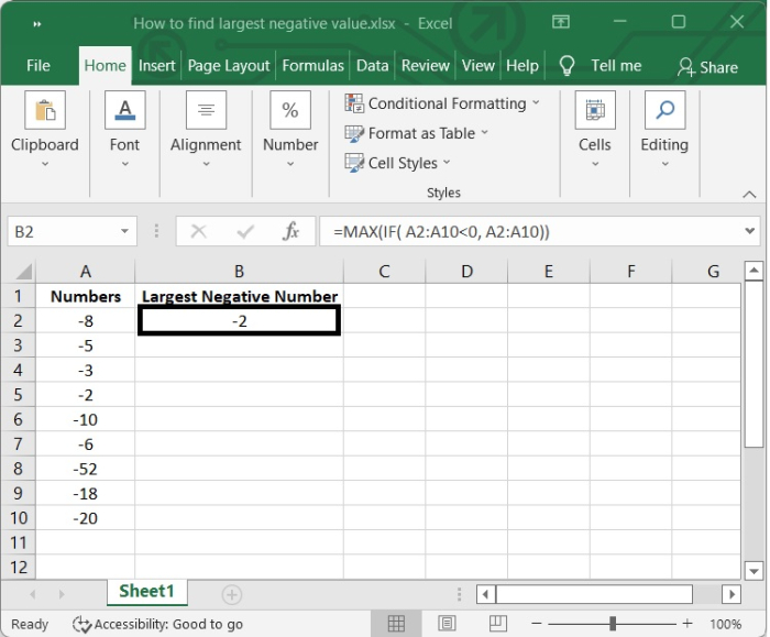
Here, we are getting "-2" as the result, which is largest negative number in the list.

Conclusion

In this tutorial, we explained how you can find the largest negative value from a given list of values.