
Article Categories
- All Categories
-
 Data Structure
-
 Networking
-
 RDBMS
RDBMS
-
 Operating System
-
 Java
Java
-
 MS Excel
-
 iOS
iOS
-
 HTML
HTML
-
 CSS
CSS
-
 Android
-
 Python
-
 C Programming
-
 C++
C++
-
 C#
C#
-
 MongoDB
-
 MySQL
MySQL
-
 Javascript
-
 PHP
PHP
-
 Economics & Finance
How To Drop The Lowest Grade And Get The Average Or Total Of Values In Excel?
Excel is a strong data analysis tool, and knowing how to alter your data to get correct results is critical. In this article, we'll show you how to use Excel's built?in functions to remove the lowest grade from a set of data and determine the average or total of the remaining numbers. This video will offer you with the knowledge and skills to efficiently handle your data, whether you are a student managing your grades or a professional working with data sets. By removing the lowest grade, you may concentrate on overall performance without being influenced by outliers or errors.
Calculating the average or total of the remaining numbers will also provide you with a clear representation of the data's central tendency or cumulative sum. So, let's get started and learn how to drop the lowest grade and execute Excel calculations to get accurate and useful results!
Drop The Lowest Grade And Get The Average Or Total Of Values
Here we will use the formula for every value, then use the auto handle to complete the task. So let us see a simple process to see how you can drop the lowest grade and get the average or total of values in Excel.
Step 1
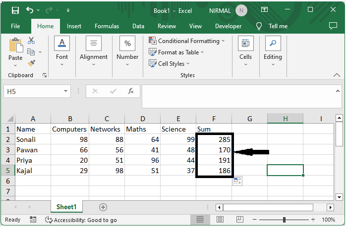
Consider an Excel sheet where the data in the sheet is similar to the below image.

First, to calculate the sum by dropping the lowest value, click on an empty cell and enter the formula as =(SUM(B2:E2)?SMALL(B2:E2,1))and drag to fill all values.
Empty cell > Formula > Enter > Drag.
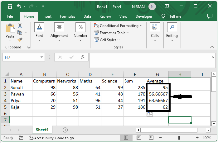
Note?
To average the data by dropping the lowest value, use the formula as follows:
=(SUM(B2:E2)?SMALL(B2:E2,1))/(COUNT(B2:E2)?1).
Conclusion
In this tutorial, we have used a simple example to demonstrate how you can drop the lowest grade and get the average or total of values in Excel to highlight a particular set of data.

8K+ Views
