How to conduct z-Test: Two Sample for Means?

In this article, we will learn how to conduct a z-test for the two independent samples in MS Excel. The main goal of the z-test is to examine the means of two independent samples. With the help of the Data Analysis option built in MS Excel, the user finds the summarized value through the z-test and reaches to the conclusion whether to reject the null hypothesis or accept the null hypothesis, the users utilize the p-value after performing the z-test.

• Null Hypothesis − There would be no relevant difference between the mean of heart patients and the Hypertension patients

• Alternative Hypothesis − There would be a relevant difference between the mean of heart patients and the Hypertension patients.

To conduct z-test for two samples

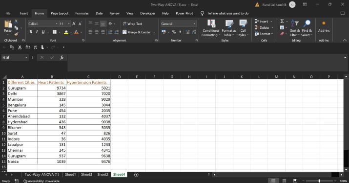
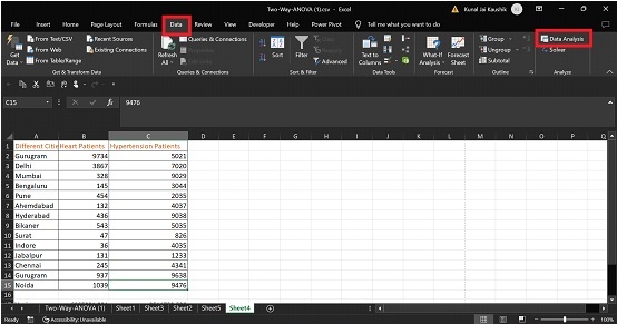
Consider the sample dataset that describes the number of Heart attack patients and the number of Hypertension patients residing in various cities.

• Step 1 − Create the dataset in the worksheet, the first column indicates the name of multiple cities, the second column contains the first sample data containing the number of Heart patients and the third column indicates the second sample information representing the number of Hypertension Patients. We must calculate the variance of distinct samples before applying the z-test.

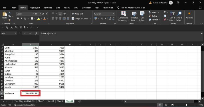
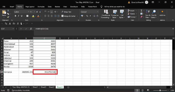
• Step 2 − Calculate the variance of the first sample. Write the formula =VAR.S(B2:B15) in the B17 cell as depicted below −

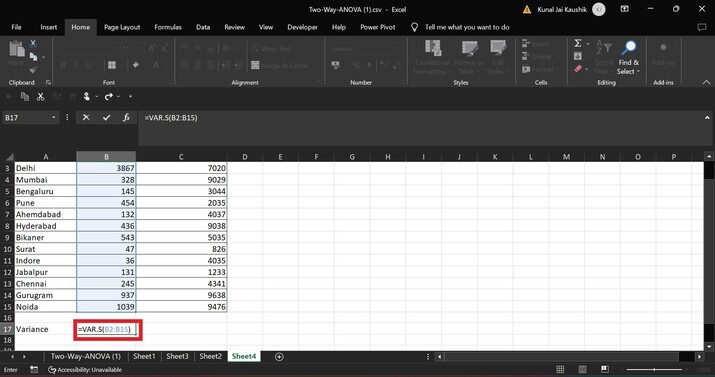
And then press Enter to obtain the variance of the specified dataset.

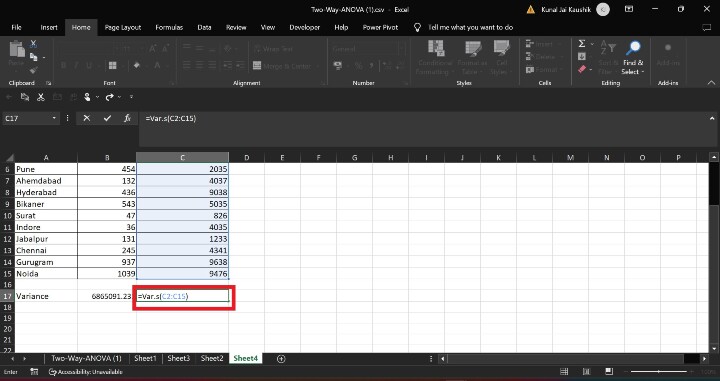
• Step 3 − Similarly, evaluate the variance of the second sample. Enter the variance formula =VAR.S(C2:C15) and press the Enter button.

• Step 4 − Choose the option named Data Analysis from the Data tab as shown in below image −

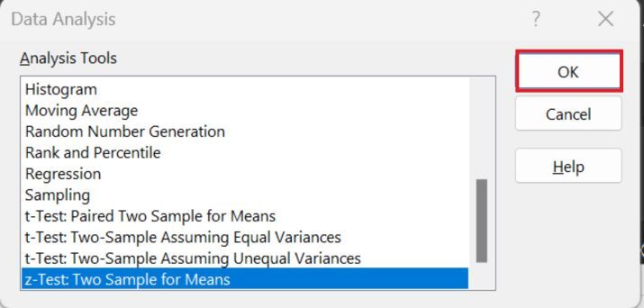
• Step 5 − Another dialog box named Data Analysis will appear. Select the z-Test: Two Sample for Means from the drop-down menu of this dialog box and then press the OK button.

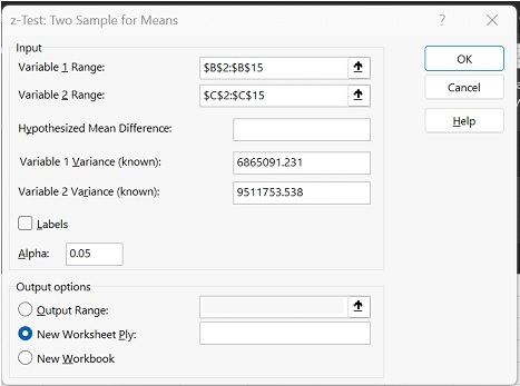
• Step 6 − Write the range of the first dataset and second dataset in the front of the Variable 1 Range and Variable 2 Range labels. Enter the values of variance 1 and variance 2 that we have calculated in step 2 and step 3. Set the value of Alpha to 0.05. Under the Output options section, users may select any of the options. Here, we choose the New Worksheet Ply: option which means the output will be generated in the new worksheet.

• Step 7 − Therefore, the output is displayed in the new worksheet named sheet 5.

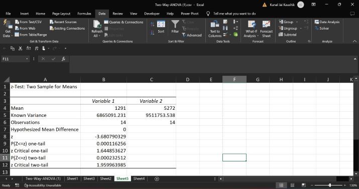
After the observation of the z-test table, P(Z<=z) one tail value that is 0.000116256 is less than 0.05, and also P(Z<=z) two-tail value that is 0.00023512 is less than 0.05 which means we have to accept the Alternative hypothesis and rejecting the Null Hypothesis.

Conclusion

Efficient hypothesis test is a significant way of working with Excel, especially when dealing with large and complex datasets. By leveraging Excel's built-in data analysis options like ANOVA, z-test, t-test for sample means, and various regression and correlation methods, you can quickly obtain and analyze the results without wasting time. Incorporate these techniques into your workflow to enhance your productivity and make your Excel experience more seamless and enjoyable.