How to Automatically Colour the Alternating Rows/Columns in Excel?

Sometimes you want to add different colours to the alternating rows or columns in the Excel sheet. This will make your sheet appear clearer and more understandable. This tutorial will help you understand how we can automatically colour-code alternating rows or columns in Excel. This procedure can be completed in two ways: first, through the use of tables, and second, through the use of conditional formatting.

Automatically Colour Alternating Rows/Columns Using Tables

Here, we will first create the table for the existing data and then select the layout to complete the task. Let us see a straightforward process to know how we can automatically colour-code alternating rows or columns using the tables. In tables, the alternate rows will be distinct color, but here we will see it more clearly.

Step 1

Let us consider an Excel sheet where the data is like the data shown in the below image.

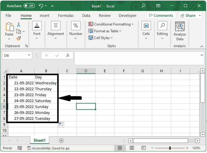
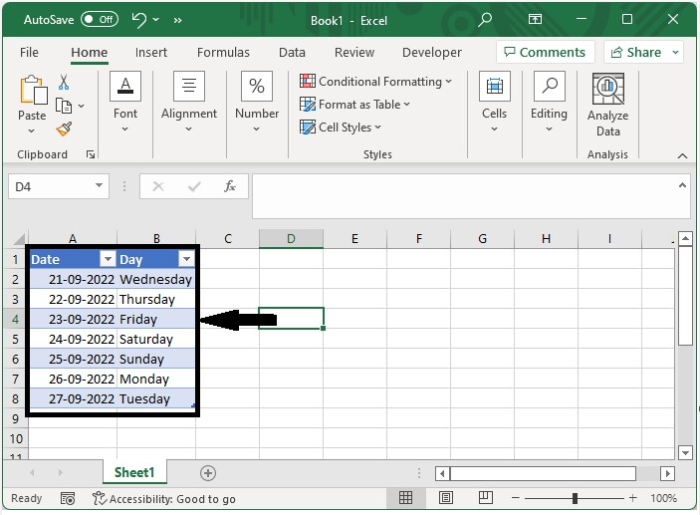
To insert the table, select the data, click insert, click table, and select the range, and our table will be successfully created, as shown in the image below.

Step 2

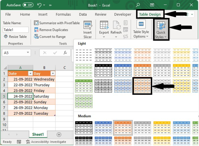
Now click on any cell of the table, then click on table design and select any style under quick styles, as shown in the below image. If you are unable to see the alternate colours, select banded rows under the table style options.

Step 3

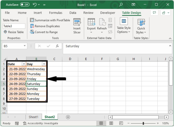
Now to get the alternate colour columns, select the banded columns under the table style options, and we will get the alternate colour columns as shown in the below image.

Automatically Colour Alternating Rows/Columns Using Conditional Formatting

Here we will use the formula for conditional formatting. Let us see an effortless process to understand how we can add an alternate row or column colour using conditional formatting in Excel.

Step 1

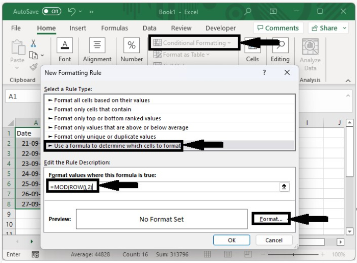
Let us consider the same data that we used in the above example. Now click on conditional formatting under "Home" and select "New Rule" to open a pop-up. In the pop-up window, click on "Use the formula" and enter the formula as =MOD(ROW(),2), then click on "Format."

Step 2

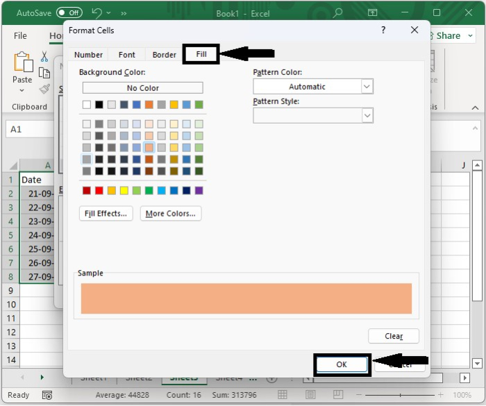
Then, click fill, choose the colour you want to use, and press OK twice.

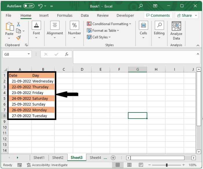
Our output of alternate rows will look like the below image.

Step 3

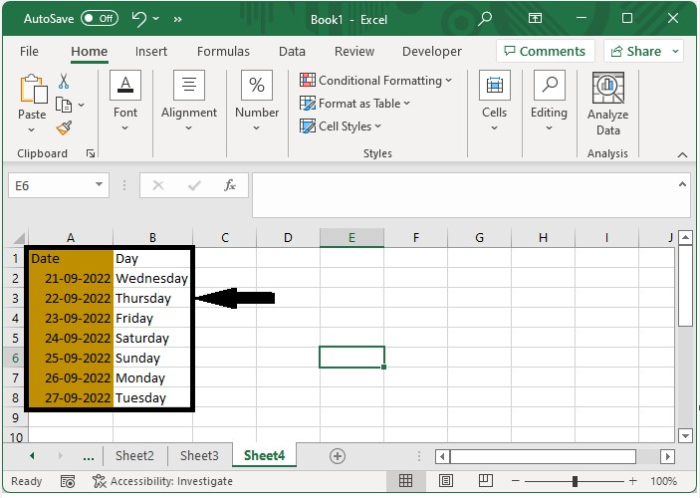
If you want a different column, then you can use the formula =MOD(COLUMN(),2)

Conclusion

In this tutorial, we used a simple example to demonstrate how we can automatically colour the alternating rows and columns in Excel.