How to Auto-Update a Chart after Entering New Data in Excel?

When we have an existing chart and you need to add new data or update the existing data, this can be done by manually updating the chart, but it can be a time-consuming process. In this tutorial, I will explain the method that saves you time. This tutorial will help you understand how we can automatically update a chart after entering new data in Excel. This can be done in two ways: first, by using the tables, and second, by using the dynamic formula.

Auto-Update a Chart after Entering New Data Using Tables

Here we will convert our data into a table to complete our task. Let us see a simple process to understand how we can automatically update a chart after entering new data using the tables.

Step 1

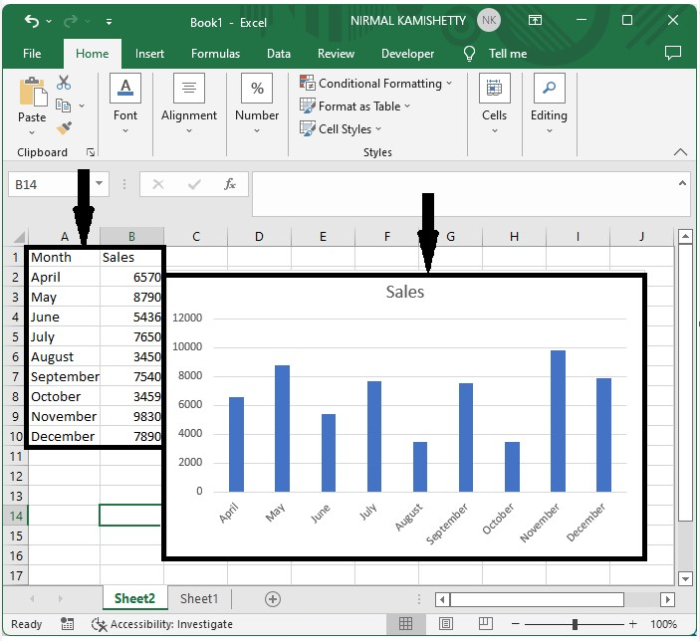
Let us consider that we have an Excel sheet that contains a chart and our new data, as shown in the below image.

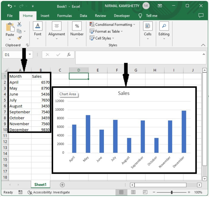
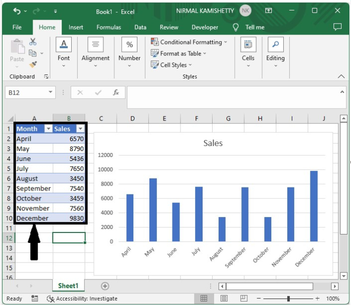
Now create a table for the data to create the table, select the data by clicking on the inset and selecting table, and select the range to create the table as shown in the below image.

Step 2

Now, every time we add data to the table, the chart will be updated automatically.

Auto-Update a Chart after Entering New Data Using Dynamic Formula

Here we will use the formula and edit the series. Let us see a simple process to understand how we can update a chart by entering new data into the dynamic formula.

Step 1

Now consider a new Excel chart. Click on formulas and select defined names to open a pop-up window, as shown in the below image. In the new pop-up type, name the month, scope sheet 2, and finally refer to =OFFSET($A$2,0,0,COUNTA($A:$A)-1).

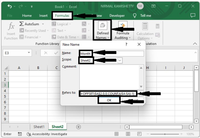
Then, for the second column, repeat the process using the formula: =OFFSET($B$2,0,0,COUNTA($B:$B)-1) .

Step 2

Then enter your data into the sheet as shown in below image.

Step 3

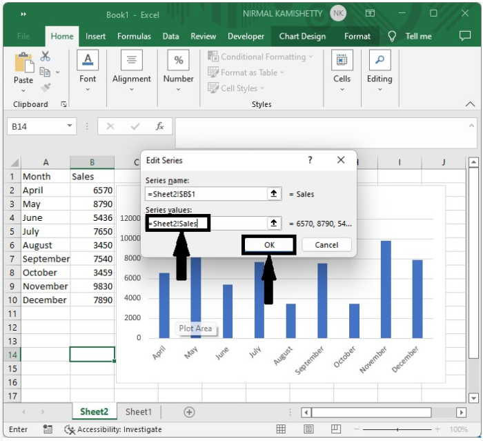
To open a new popup, right-click on any of the bars and select data. Change the series values to =Sheet2!Sales in the pop-up window under Legend Entries, then click OK.

Step 4

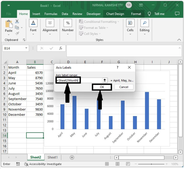
Now, under the horizontal value, click edit and change the axis label range to =Sheet2!Month, then OK, and then on again.

Step 5

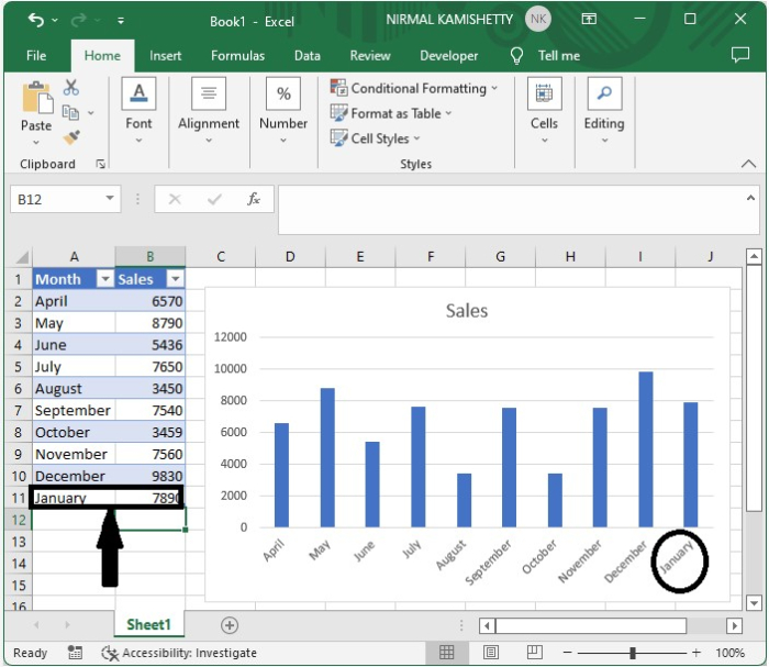
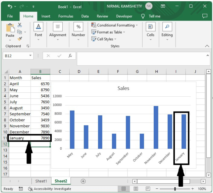
Finally, when we add the new values to the list, our chart will update automatically, as shown in the below image.

Conclusion

In this tutorial, we used a simple example to demonstrate how you can autoupdate a chart after entering new data in Excel.