
Article Categories
- All Categories
-
 Data Structure
-
 Networking
-
 RDBMS
RDBMS
-
 Operating System
-
 Java
Java
-
 MS Excel
-
 iOS
iOS
-
 HTML
HTML
-
 CSS
CSS
-
 Android
-
 Python
-
 C Programming
-
 C++
C++
-
 C#
C#
-
 MongoDB
-
 MySQL
MySQL
-
 Javascript
-
 PHP
PHP
-
 Economics & Finance
How to Apply Colour Banded Rows or Columns in Excel?
When we are using Excel, we want to add different colours to cells to create a design that can improve the neatness of the data. This also makes the excel sheet look nicer and allows for faster data analysis. This article will help you understand how we can apply color-banded rows or columns in Excel. This can be done using a simple method in Excel by using conditional formatting and applying different colours. Read this tutorial to learn a simple process to apply color-banded rows or columns in Excel.
Applying Colour Banded Rows or Columns Using Conditional Formatting
Here, we will first give the condition and select the colour we want to apply. Let us see a simple process to understand how we can add color-banded rows or columns in Excel using conditional formatting in a simple process.
Step 1
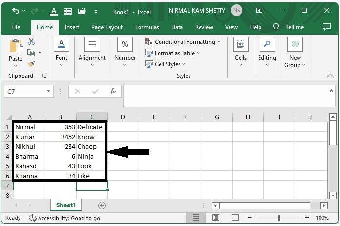
Assume we have an excel sheet with data similar to the data shown in the screenshot below.
Now to add the banded rows, select the data, then select the new rule under conditional formatting, which is present in the Excel Home Ribbon, and a new pop-up window will be opened.
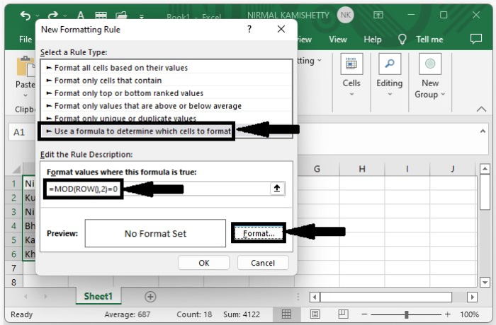
In the new pop-up, click on "Use a Formula," then enter the formula as =MOD(ROW(),2)=0 in the formula box, and click on "Format" to open a new pop-up.
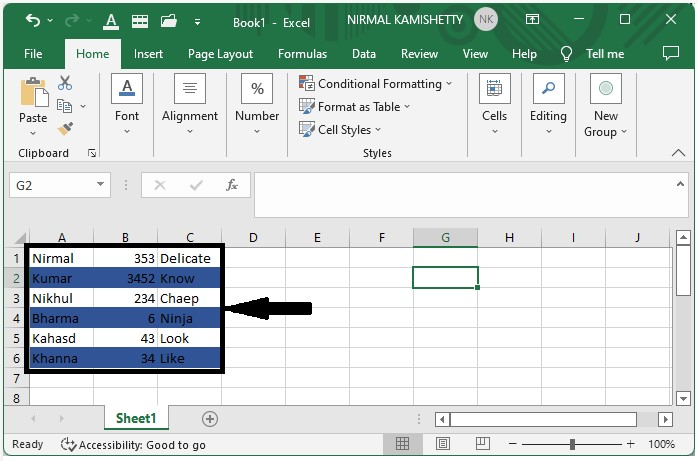
Step 2
In the new pop-up window, click "Fill" and choose a color, then click "OK" to get the banded rows shown in the image below.
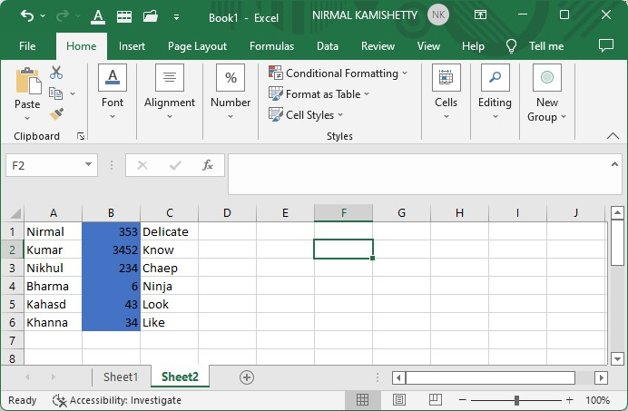
Step 3
Now to add the banded column, use the formula =MOD(COLUMN(), 2)=0in the formula box and click OK in step one and our result will be similar to the below image
Conclusion
In this tutorial, we used a simple example to demonstrate how you can apply color-banded rows or columns in Excel to highlight a particular set of data.

466 Views
