
Article Categories
- All Categories
-
 Data Structure
-
 Networking
-
 RDBMS
RDBMS
-
 Operating System
-
 Java
Java
-
 MS Excel
-
 iOS
iOS
-
 HTML
HTML
-
 CSS
CSS
-
 Android
-
 Python
-
 C Programming
-
 C++
C++
-
 C#
C#
-
 MongoDB
-
 MySQL
MySQL
-
 Javascript
-
 PHP
PHP
-
 Economics & Finance
How to Always Show an Arrow of Data Validation List in Excel?
When we are using a drop-down list in Excel, the arrow mark of the drop-down list will only appear if we click on any cell of the list. This creates a problem when we are using multiple drop-down lists in a single column. We can solve this problem by adding a persistent arrow mark to the cell in Excel. This tutorial will help you understand how we can show the arrow of a data validation list in Excel.
Showing the Arrow of Data Validation List in Excel
Here we will first use the data validation list and then inset an arrow symbol in the cell adjacent to the list. Let us see a simple process to add an arrow to the drop-down list in Excel by following a simple process as described below.
Step 1
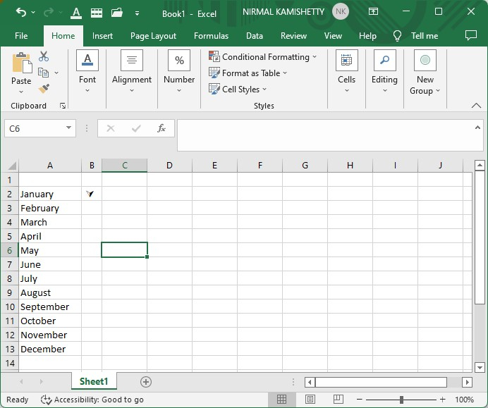
Consider the Excel sheet with data similar to the data shown in the image below.
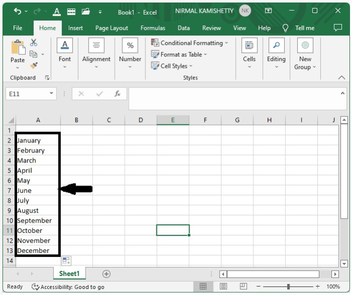
To complete our task in a simpler way, keep the first cell empty.
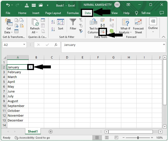
Now to create the data validation list, click on data validation under the data in the Excel ribbon, then select allow in the list and all the cells as sources, and click on OK to create the list as shown in the below figure.
Step 2
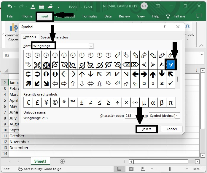
Click on the cell that is right for the top cell of the drop-down list, then select Insert, then select Symbols and select an arrow mark under wings from the drop-down list as represented in the below image, then click on Insert and close the pop-up window.
Step 3
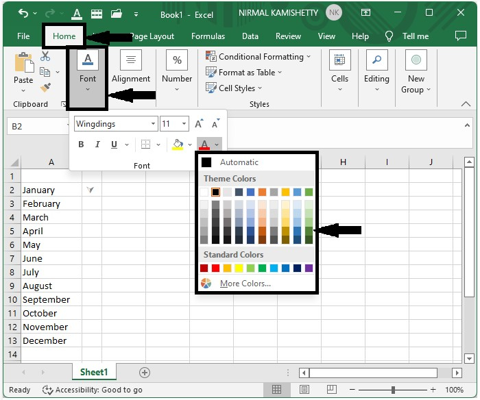
Now, resize the cell where the arrow mark is present equal to the arrow mark shown for the drop-down list, and then select the grey colour by clicking on the font under "home" in the Excel ribbon, as shown in the below image.
Then our final result will be similar to the image shown below.
Conclusion
In this tutorial, we used a simple example to demonstrate how you can always show an arrow for data validation lists in Excel to highlight a particular set of data.

16K+ Views
