
Article Categories
- All Categories
-
 Data Structure
-
 Networking
-
 RDBMS
RDBMS
-
 Operating System
-
 Java
Java
-
 MS Excel
-
 iOS
iOS
-
 HTML
HTML
-
 CSS
CSS
-
 Android
-
 Python
-
 C Programming
-
 C++
C++
-
 C#
C#
-
 MongoDB
-
 MySQL
MySQL
-
 Javascript
-
 PHP
PHP
-
 Economics & Finance
How to Add Percentage of Grand Total/Subtotal Column in an Excel Pivot Table?
When we create a pivot table in excel where there is a list of items and you want to know their share in the list in percentage. Read through this tutorial to understand how you can create a new column where it shows the percentage of grand total or subtotal column in a excel pivot table in a simple process.
How to Add Percentage of Grand Total Column in Excel Pivot Table
Let us see a simple process to add percentage column of total column in an Excel pivot table ?
Step 1
Let us assume the Excel sheet where the data is represented looks similar to the screenshot given below ?
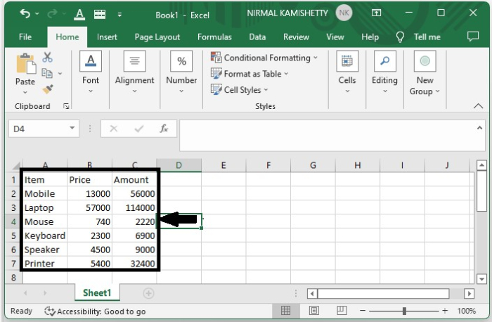
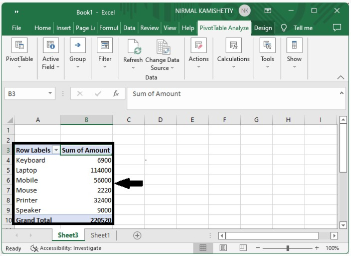
To create a pivot table, select "Data" and select "Pivot Table" under "Insert" and the pivot table will be created successfully as shown in the following image. Create the pivot table for Item and Amount.
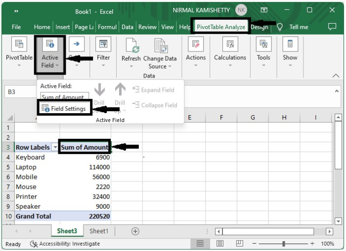
Step 2
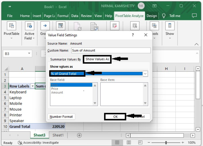
Now click the "Sum of Amount" and click "Field Settings" under "Active Field" under "Pivot Table Analyze", and then a new pop up will be opened as shown in the following image ?
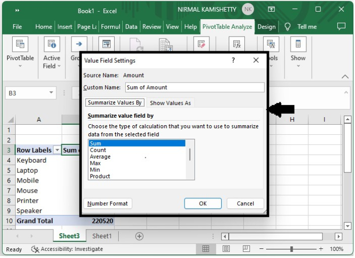
Step 3
Now click the "Show Values" and then select "% of grand total" from the drop-down list of "Show Value As" and finally click "OK".
Our final result will look similar to the following image ?
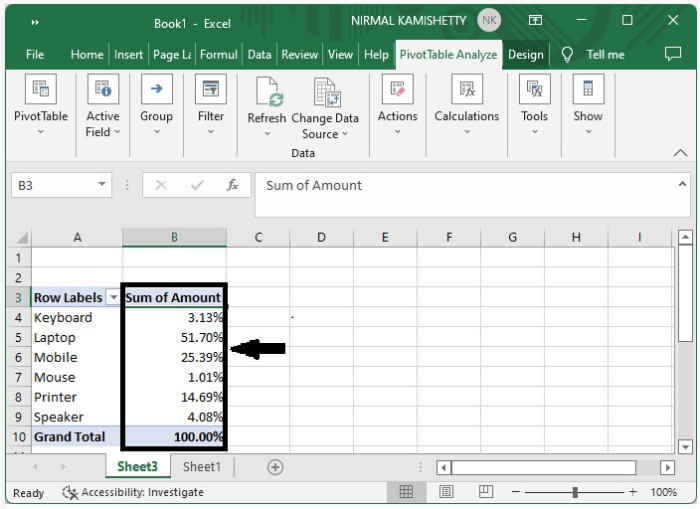
We can also change the name as percentage of amount and if you want to retain the before column, just make a duplicate column for it in the pivot table.
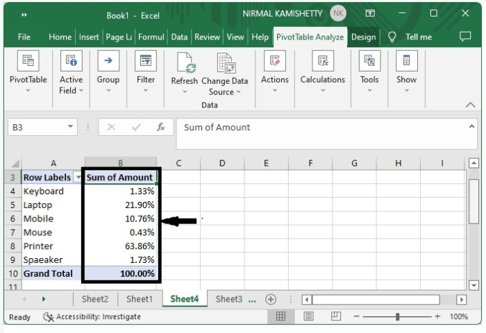
How to Add Percentage of Sub Total Column in Pivot Table
Repeat the same process till Step 2 in the above example and then follow this. Select the show value as % of parent row total. Our final result will look similar to the following image ?
This is how we can add percentage of grand total/subtotal column in an Excel pivot table.

4K+ Views
