
Article Categories
- All Categories
-
 Data Structure
-
 Networking
-
 RDBMS
RDBMS
-
 Operating System
-
 Java
Java
-
 MS Excel
-
 iOS
iOS
-
 HTML
HTML
-
 CSS
CSS
-
 Android
-
 Python
-
 C Programming
-
 C++
C++
-
 C#
C#
-
 MongoDB
-
 MySQL
MySQL
-
 Javascript
-
 PHP
PHP
-
 Economics & Finance
How to Add a Hyperlink to a Specific Part of a Cell in Excel?
When we create a hyperlink in Excel, the whole cell will work as a hyperlink. There is no way we can make the part of the cell work as a hyperlink. But I will explain a simple trick to see that a hyperlink is created for part of a cell. On a website, a hyperlink (or link) is an item like a word or button that points to another location. When you click on a link, the link will take you to the target of the link, which may be a webpage, document, or other online content. Websites use hyperlinks as a way to navigate online content.
This tutorial will help you understand how we can add hyperlinks to specific parts of cells in Excel. We can do it by changing the font colour of the cell values.
Adding a Hyperlink to a Specific Part of a Cell
Here we will change the font and colour of part of the data where you want to remove the hyperlink. Let's go over a simple procedure for adding hyperlinks to specific parts of cells in Excel by changing the font color.
Step 1
Let us consider an Excel sheet where we have a hyperlink similar to the below image.
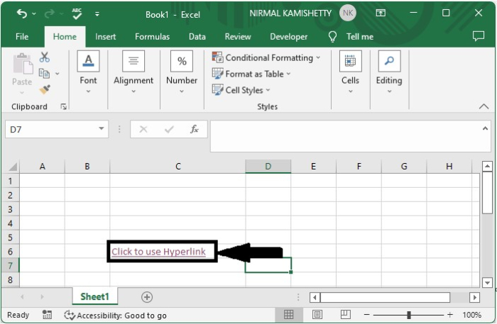
If you need to create the hyperlink, click on the cell and use the command CTRL + H, enter the address you want to link, and click OK.
Click > CTRL + H > Address > OK
Step 2
Now click on the cell and select the data you don?t want to use as a hyperlink, then click on font and change the font colour to black.
Cell > Select data > Font > Font colour > Black
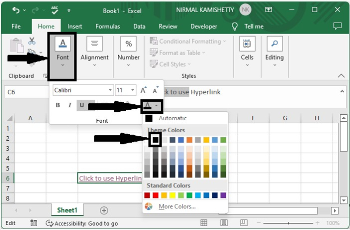
The unselected data will then be displayed successfully as a hyper link.
Conclusion
In this tutorial, we used a simple example to demonstrate how we can add hyperlinks to specific parts of cells in Excel to highlight particular sets of data. The hyperlink will work for the whole cell as before, but there is a difference in cell visibility.

12K+ Views
