- Gensim - Home
- Gensim - Introduction
- Gensim - Getting Started
- Gensim - Documents & Corpus
- Gensim - Vector & Model
- Gensim - Creating a Dictionary
- Creating a bag of words (BoW) Corpus
- Gensim - Transformations
- Gensim - Creating TF-IDF Matrix
- Gensim - Topic Modeling
- Gensim - Creating LDA Topic Model
- Gensim - Using LDA Topic Model
- Gensim - Creating LDA Mallet Model
- Gensim - Documents & LDA Model
- Gensim - Creating LSI & HDP Topic Model
- Gensim - Developing Word Embedding
- Gensim - Doc2Vec Model
- Gensim Useful Resources
- Gensim - Quick Guide
- Gensim - Useful Resources
- Gensim - Discussion
Gensim - Quick Guide
Gensim - Introduction
This chapter will help you understand history and features of Gensim along with its uses and advantages.
What is Gensim?
Gensim = Generate Similar is a popular open source natural language processing (NLP) library used for unsupervised topic modeling. It uses top academic models and modern statistical machine learning to perform various complex tasks such as −
- Building document or word vectors
- Corpora
- Performing topic identification
- Performing document comparison (retrieving semantically similar documents)
- Analysing plain-text documents for semantic structure
Apart from performing the above complex tasks, Gensim, implemented in Python and Cython, is designed to handle large text collections using data streaming as well as incremental online algorithms. This makes it different from those machine learning software packages that target only in-memory processing.
History
In 2008, Gensim started off as a collection of various Python scripts for the Czech Digital Mathematics. There, it served to generate a short list of the most similar articles to a particular given article. But in 2009, RARE Technologies Ltd. released its initial release. Then, later in July 2019, we got its stable release (3.8.0).
Various Features
Following are some of the features and capabilities offered by Gensim −
Scalability
Gensim can easily process large and web-scale corpora by using its incremental online training algorithms. It is scalable in nature, as there is no need for the whole input corpus to reside fully in Random Access Memory (RAM) at any one time. In other words, all its algorithms are memory-independent with respect to the corpus size.
Robust
Gensim is robust in nature and has been in use in various systems by various people as well as organisations for over 4 years. We can easily plug in our own input corpus or data stream. It is also very easy to extend with other Vector Space Algorithms.
Platform Agnostic
As we know that Python is a very versatile language as being pure Python Gensim runs on all the platforms (like Windows, Mac OS, Linux) that supports Python and Numpy.
Efficient Multicore Implementations
In order to speed up processing and retrieval on machine clusters, Gensim provides efficient multicore implementations of various popular algorithms like Latent Semantic Analysis (LSA), Latent Dirichlet Allocation (LDA), Random Projections (RP), Hierarchical Dirichlet Process (HDP).
Open Source and Abundance of Community Support
Gensim is licensed under the OSI-approved GNU LGPL license which allows it to be used for both personal as well as commercial use for free. Any modifications made in Gensim are in turn open-sourced and has abundance of community support too.
Uses of Gensim
Gensim has been used and cited in over thousand commercial and academic applications. It is also cited by various research papers and student theses. It includes streamed parallelised implementations of the following −
fastText
fastText, uses a neural network for word embedding, is a library for learning of word embedding and text classification. It is created by Facebooks AI Research (FAIR) lab. This model, basically, allows us to create a supervised or unsupervised algorithm for obtaining vector representations for words.
Word2vec
Word2vec, used to produce word embedding, is a group of shallow and two-layer neural network models. The models are basically trained to reconstruct linguistic contexts of words.
LSA (Latent Semantic Analysis)
It is a technique in NLP (Natural Language Processing) that allows us to analyse relationships between a set of documents and their containing terms. It is done by producing a set of concepts related to the documents and terms.
LDA (Latent Dirichlet Allocation)
It is a technique in NLP that allows sets of observations to be explained by unobserved groups. These unobserved groups explain, why some parts of the data are similar. Thats the reason, it is a generative statistical model.
tf-idf (term frequency-inverse document frequency)
tf-idf, a numeric statistic in information retrieval, reflects how important a word is to a document in a corpus. It is often used by search engines to score and rank a documents relevance given a user query. It can also be used for stop-words filtering in text summarisation and classification.
All of them will be explained in detail in the next sections.
Advantages
Gensim is a NLP package that does topic modeling. The important advantages of Gensim are as follows −
We may get the facilities of topic modeling and word embedding in other packages like scikit-learn and R, but the facilities provided by Gensim for building topic models and word embedding is unparalleled. It also provides more convenient facilities for text processing.
Another most significant advantage of Gensim is that, it let us handle large text files even without loading the whole file in memory.
Gensim doesnt require costly annotations or hand tagging of documents because it uses unsupervised models.
Gensim - Getting Started
The chapter enlightens about the prerequisites for installing Gensim, its core dependencies and information about its current version.
Prerequisites
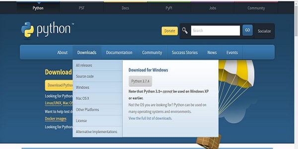
In order to install Gensim, we must have Python installed on our computers. You can go to the link www.python.org/downloads/ and select the latest version for your OS i.e. Windows and Linux/Unix. You can refer to the link www.tutorialspoint.com/python3/index.htm for basic tutorial on Python. Gensim is supported for Linux, Windows and Mac OS X.
Code Dependencies
Gensim should run on any platform that supports Python 2.7 or 3.5+ and NumPy. It actually depends on the following software −
Python
Gensim is tested with Python versions 2.7, 3.5, 3.6, and 3.7.
Numpy
As we know that, NumPy is a package for scientific computing with Python. It can also be used as an efficient multi-dimensional container of generic data. Gensim depends on NumPy package for number crunching. For basic tutorial on Python, you can refer to the link www.tutorialspoint.com/numpy/index.htm.
smart_open
smart_open, a Python 2 & Python 3 library, is used for efficient streaming of very large files. It supports streaming from/to storages such as S3, HDFS, WebHDFS, HTTP, HTTPS, SFTP, or local filesystems. Gensim depends upon smart_open Python library for transparently opening files on remote storage as well as compressed files.
Current Version
The current version of Gensim is 3.8.0 which was released in July 2019.
Installing Using Terminal
One of the simplest ways to install Gensim, is to run the following command in your terminal −
pip install --upgrade gensim
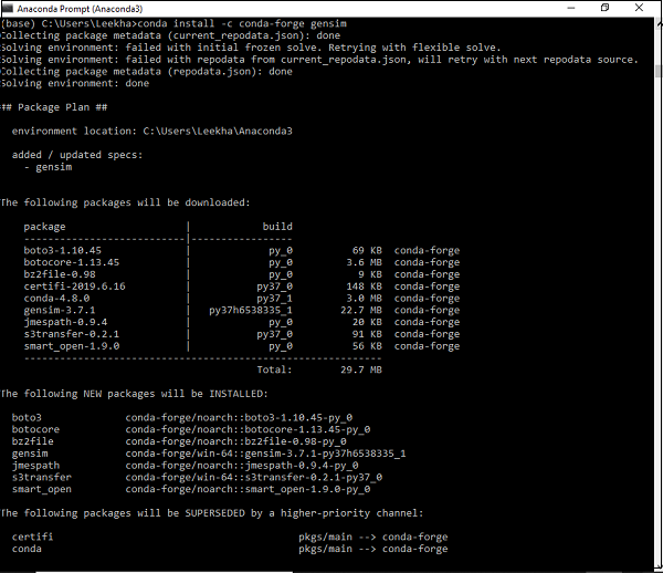
Installing Using Conda Environment
An alternative way to download Gensim is, to use conda environment. Run the following command in your conda terminal −
conda install c conda-forge gensim
Installing Using Source Package
Suppose, if you have downloaded and unzipped the source package, then you need to run the following commands −
python setup.py test
python setup.py install
Gensim - Documents & Corpus
Here, we shall learn about the core concepts of Gensim, with main focus on the documents and the corpus.
Core Concepts of Gensim
Following are the core concepts and terms that are needed to understand and use Gensim −
Document − ZIt refers to some text.
Corpus − It refers to a collection of documents.
Vector − Mathematical representation of a document is called vector.
Model − It refers to an algorithm used for transforming vectors from one representation to another.
What is Document?
As discussed, it refers to some text. If we go in some detail, it is an object of the text sequence type which is known as str in Python 3. For example, in Gensim, a document can be anything such as −
- Short tweet of 140 characters
- Single paragraph, i.e. article or research paper abstract
- News article
- Book
- Novel
- Theses
Text Sequence
A text sequence type is commonly known as str in Python 3. As we know that in Python, textual data is handled with strings or more specifically str objects. Strings are basically immutable sequences of Unicode code points and can be written in the following ways −
Single quotes − For example, Hi! How are you?. It allows us to embed double quotes also. For example, Hi! How are you?
Double quotes − For example, "Hi! How are you?". It allows us to embed single quotes also. For example, "Hi! 'How' are you?"
Triple quotes − It can have either three single quotes like, '''Hi! How are you?'''. or three double quotes like, """Hi! 'How' are you?"""
All the whitespaces will be included in the string literal.
Example
Following is an example of a Document in Gensim −
Document = Tutorialspoint.com is the biggest online tutorials library and its all free also
What is Corpus?
A corpus may be defined as the large and structured set of machine-readable texts produced in a natural communicative setting. In Gensim, a collection of document object is called corpus. The plural of corpus is corpora.
Role of Corpus in Gensim
A corpus in Gensim serves the following two roles −
Serves as Input for Training a Model
The very first and important role a corpus plays in Gensim, is as an input for training a model. In order to initialize models internal parameters, during training, the model look for some common themes and topics from the training corpus. As discussed above, Gensim focuses on unsupervised models, hence it doesnt require any kind of human intervention.
Serves as Topic Extractor
Once the model is trained, it can be used to extract topics from the new documents. Here, the new documents are the ones that are not used in the training phase.
Example
The corpus can include all the tweets by a particular person, list of all the articles of a newspaper or all the research papers on a particular topic etc.
Collecting Corpus
Following is an example of small corpus which contains 5 documents. Here, every document is a string consisting of a single sentence.
t_corpus = [
   "A survey of user opinion of computer system response time",
   "Relation of user perceived response time to error measurement",
   "The generation of random binary unordered trees",
   "The intersection graph of paths in trees",
   "Graph minors IV Widths of trees and well quasi ordering",
]
Preprocessing Collecting Corpus
Once we collect the corpus, a few preprocessing steps should be taken to keep corpus simple. We can simply remove some commonly used English words like the. We can also remove words that occur only once in the corpus.
For example, the following Python script is used to lowercase each document, split it by white space and filter out stop words −
Example
import pprint
t_corpus = [
   "A survey of user opinion of computer system response time",
   "Relation of user perceived response time to error measurement",
   "The generation of random binary unordered trees",
   "The intersection graph of paths in trees",
   "Graph minors IV Widths of trees and well quasi ordering",
]
stoplist = set('for a of the and to in'.split(' '))
processed_corpus = [[word for word in document.lower().split() if word not in stoplist]
   for document in t_corpus]

pprint.pprint(processed_corpus)
]
Output
[['survey', 'user', 'opinion', 'computer', 'system', 'response', 'time'],
['relation', 'user', 'perceived', 'response', 'time', 'error', 'measurement'],
['generation', 'random', 'binary', 'unordered', 'trees'],
['intersection', 'graph', 'paths', 'trees'],
['graph', 'minors', 'iv', 'widths', 'trees', 'well', 'quasi', 'ordering']]
Effective Preprocessing
Gensim also provides function for more effective preprocessing of the corpus. In such kind of preprocessing, we can convert a document into a list of lowercase tokens. We can also ignore tokens that are too short or too long. Such function is gensim.utils.simple_preprocess(doc, deacc=False, min_len=2, max_len=15).
gensim.utils.simple_preprocess() fucntion
Gensim provide this function to convert a document into a list of lowercase tokens and also for ignoring tokens that are too short or too long. It has the following parameters −
doc(str)
It refers to the input document on which preprocessing should be applied.
deacc(bool, optional)
This parameter is used to remove the accent marks from tokens. It uses deaccent() to do this.
min_len(int, optional)
With the help of this parameter, we can set the minimum length of a token. The tokens shorter than defined length will be discarded.
max_len(int, optional)
With the help of this parameter we can set the maximum length of a token. The tokens longer than defined length will be discarded.
The output of this function would be the tokens extracted from input document.
Gensim - Vector & Model
Here, we shall learn about the core concepts of Gensim, with main focus on the vector and the model.
What is Vector?
What if we want to infer the latent structure in our corpus? For this, we need to represent the documents in a such a way that we can manipulate the same mathematically. One popular kind of representation is to represent every document of corpus as a vector of features. Thats why we can say that vector is a mathematical convenient representation of a document.
To give you an example, lets represent a single feature, of our above used corpus, as a Q-A pair −
Q − How many times does the word Hello appear in the document?
A − Zero(0).
Q − How many paragraphs are there in the document?
A − Two(2)
The question is generally represented by its integer id, hence the representation of this document is a series of pairs like (1, 0.0), (2, 2.0). Such vector representation is known as a dense vector. Why dense, because it comprises an explicit answer to all the questions written above.
The representation can be a simple like (0, 2), if we know all the questions in advance. Such sequence of the answers (of course if the questions are known in advance) is the vector for our document.
Another popular kind of representation is the bag-of-word (BoW) model. In this approach, each document is basically represented by a vector containing the frequency count of every word in the dictionary.
To give you an example, suppose we have a dictionary that contains the words [Hello, How, are, you]. A document consisting of the string How are you how would then be represented by the vector [0, 2, 1, 1]. Here, the entries of the vector are in order of the occurrences of Hello, How, are, and you.
Vector Versus Document
From the above explanation of vector, the distinction between a document and a vector is almost understood. But, to make it clearer, document is text and vector is a mathematically convenient representation of that text. Unfortunately, sometimes many people use these terms interchangeably.
For example, suppose we have some arbitrary document A then instead of saying, the vector that corresponds to document A, they used to say, the vector A or the document A. This leads to great ambiguity. One more important thing to be noted here is that, two different documents may have the same vector representation.
Converting corpus into list of vectors
Before taking an implementation example of converting corpus into the list of vectors, we need to associate each word in the corpus with a unique integer ID. For this, we will be extending the example taken in above chapter.
Example
from gensim import corpora
dictionary = corpora.Dictionary(processed_corpus)
print(dictionary)
Output
Dictionary(25 unique tokens: ['computer', 'opinion', 'response', 'survey', 'system']...)
It shows that in our corpus there are 25 different tokens in this gensim.corpora.Dictionary.
Implementation Example
We can use the dictionary to turn tokenised documents into these 5-diemsional vectors as follows −
pprint.pprint(dictionary.token2id)
Output
{
   'binary': 11,
   'computer': 0,
   'error': 7,
   'generation': 12,
   'graph': 16,
   'intersection': 17,
   'iv': 19,
   'measurement': 8,
   'minors': 20,
   'opinion': 1,
   'ordering': 21,
   'paths': 18,
   'perceived': 9,
   'quasi': 22,
   'random': 13,
   'relation': 10,
   'response': 2,
   'survey': 3,
   'system': 4,
   'time': 5,
   'trees': 14,
   'unordered': 15,
   'user': 6,
   'well': 23,
   'widths': 24
}
And similarly, we can create the bag-of-word representation for a document as follows −
BoW_corpus = [dictionary.doc2bow(text) for text in processed_corpus]
pprint.pprint(BoW_corpus)
Output
[
   [(0, 1), (1, 1), (2, 1), (3, 1), (4, 1), (5, 1), (6, 1)],
   [(2, 1), (5, 1), (6, 1), (7, 1), (8, 1), (9, 1), (10, 1)],
   [(11, 1), (12, 1), (13, 1), (14, 1), (15, 1)],
   [(14, 1), (16, 1), (17, 1), (18, 1)],
   [(14, 1), (16, 1), (19, 1), (20, 1), (21, 1), (22, 1), (23, 1), (24, 1)]
]
What is Model?
Once we have vectorised the corpus, next what? Now, we can transform it using models. Model may be referred to an algorithm used for transforming one document representation to other.
As we have discussed, documents, in Gensim, are represented as vectors hence, we can, though model as a transformation between two vector spaces. There is always a training phase where models learn the details of such transformations. The model reads the training corpus during training phase.
Initializing a Model
Lets initialise tf-idf model. This model transforms vectors from the BoW (Bag of Words) representation to another vector space where the frequency counts are weighted according to the relative rarity of every word in corpus.
Implementation Example
In the following example, we are going to initialise the tf-idf model. We will train it on our corpus and then transform the string trees graph.
Example
from gensim import models
tfidf = models.TfidfModel(BoW_corpus)
words = "trees graph".lower().split()
print(tfidf[dictionary.doc2bow(words)])
Output
[(3, 0.4869354917707381), (4, 0.8734379353188121)]
Now, once we created the model, we can transform the whole corpus via tfidf and index it, and query the similarity of our query document (we are giving the query document trees system) against each document in the corpus −
Example
from gensim import similarities
index = similarities.SparseMatrixSimilarity(tfidf[BoW_corpus],num_features=5)
query_document = 'trees system'.split()
query_bow = dictionary.doc2bow(query_document)
simils = index[tfidf[query_bow]]
print(list(enumerate(simils)))
Output
[(0, 0.0), (1, 0.0), (2, 1.0), (3, 0.4869355), (4, 0.4869355)]
From the above output, document 4 and document 5 has a similarity score of around 49%.
Moreover, we can also sort this output for more readability as follows −
Example
for doc_number, score in sorted(enumerate(sims), key=lambda x: x[1], reverse=True):
   print(doc_number, score)
Output
2 1.0
3 0.4869355
4 0.4869355
0 0.0
1 0.0
Gensim - Creating a Dictionary
In last chapter where we discussed about vector and model, you got an idea about the dictionary. Here, we are going to discuss Dictionary object in a bit more detail.
What is Dictionary?
Before getting deep dive into the concept of dictionary, lets understand some simple NLP concepts −
Token − A token means a word.
Document − A document refers to a sentence or paragraph.
Corpus − It refers to a collection of documents as a bag of words (BoW).
For all the documents, a corpus always contains each words tokens id along with its frequency count in the document.
Lets move to the concept of dictionary in Gensim. For working on text documents, Gensim also requires the words, i.e. tokens to be converted to their unique ids. For achieving this, it gives us the facility of Dictionary object, which maps each word to their unique integer id. It does this by converting input text to the list of words and then pass it to the corpora.Dictionary() object.
Need of Dictionary
Now the question arises that what is actually the need of dictionary object and where it can be used? In Gensim, the dictionary object is used to create a bag of words (BoW) corpus which further used as the input to topic modelling and other models as well.
Forms of Text Inputs
There are three different forms of input text, we can provide to Gensim −
As the sentences stored in Pythons native list object (known as str in Python 3)
As one single text file (can be small or large one)
Multiple text files
Creating a Dictionary Using Gensim
As discussed, in Gensim, the dictionary contains the mapping of all words, a.k.a tokens to their unique integer id. We can create a dictionary from list of sentences, from one or more than one text files (text file containing multiple lines of text). So, first lets start by creating dictionary using list of sentences.
From a List of Sentences
In the following example we will be creating dictionary from a list of sentences. When we have list of sentences or you can say multiple sentences, we must convert every sentence to a list of words and comprehensions is one of the very common ways to do this.
Implementation Example
First, import the required and necessary packages as follows −
import gensim
from gensim import corpora
from pprint import pprint
Next, make the comprehension list from list of sentences/document to use it creating the dictionary −
doc = [
   "CNTK formerly known as Computational Network Toolkit",
   "is a free easy-to-use open-source commercial-grade toolkit",
   "that enable us to train deep learning algorithms to learn like the human brain."
]
Next, we need to split the sentences into words. It is called tokenisation.
text_tokens = [[text for text in doc.split()] for doc in doc]
Now, with the help of following script, we can create the dictionary −
dict_LoS = corpora.Dictionary(text_tokens)
Now lets get some more information like number of tokens in the dictionary −
print(dict_LoS)
Output
Dictionary(27 unique tokens: ['CNTK', 'Computational', 'Network', 'Toolkit', 'as']...)
We can also see the word to unique integer mapping as follows −
print(dict_LoS.token2id)
Output
{
   'CNTK': 0, 'Computational': 1, 'Network': 2, 'Toolkit': 3, 'as': 4,
   'formerly': 5, 'known': 6, 'a': 7, 'commercial-grade': 8, 'easy-to-use': 9,
   'free': 10, 'is': 11, 'open-source': 12, 'toolkit': 13, 'algorithms': 14,
   'brain.': 15, 'deep': 16, 'enable': 17, 'human': 18, 'learn': 19, 'learning': 20,
   'like': 21, 'that': 22, 'the': 23, 'to': 24, 'train': 25, 'us': 26
}
Complete Implementation Example
import gensim
from gensim import corpora
from pprint import pprint
doc = [
   "CNTK formerly known as Computational Network Toolkit",
   "is a free easy-to-use open-source commercial-grade toolkit",
   "that enable us to train deep learning algorithms to learn like the human brain."
]
text_tokens = [[text for text in doc.split()] for doc in doc]
dict_LoS = corpora.Dictionary(text_tokens)
print(dict_LoS.token2id)
From Single Text File
In the following example we will be creating dictionary from a single text file. In the similar fashion, we can also create dictionary from more than one text files (i.e. directory of files).
For this, we have saved the document, used in previous example, in the text file named doc.txt. Gensim will read the file line by line and process one line at a time by using simple_preprocess. In this way, it doesnt need to load the complete file in memory all at once.
Implementation Example
First, import the required and necessary packages as follows −
import gensim
from gensim import corpora
from pprint import pprint
from gensim.utils import simple_preprocess
from smart_open import smart_open
import os
Next line of codes will make gensim dictionary by using the single text file named doc.txt −
dict_STF = corpora.Dictionary(
   simple_preprocess(line, deacc =True) for line in open(doc.txt, encoding=utf-8)
)
Now lets get some more information like number of tokens in the dictionary −
print(dict_STF)
Output
Dictionary(27 unique tokens: ['CNTK', 'Computational', 'Network', 'Toolkit', 'as']...)
We can also see the word to unique integer mapping as follows −
print(dict_STF.token2id)
Output
{
   'CNTK': 0, 'Computational': 1, 'Network': 2, 'Toolkit': 3, 'as': 4,
   'formerly': 5, 'known': 6, 'a': 7, 'commercial-grade': 8, 'easy-to-use': 9,
   'free': 10, 'is': 11, 'open-source': 12, 'toolkit': 13, 'algorithms': 14,
   'brain.': 15, 'deep': 16, 'enable': 17, 'human': 18, 'learn': 19,
   'learning': 20, 'like': 21, 'that': 22, 'the': 23, 'to': 24, 'train': 25, 'us': 26
}
Complete Implementation Example
import gensim
from gensim import corpora
from pprint import pprint
from gensim.utils import simple_preprocess
from smart_open import smart_open
import os
dict_STF = corpora.Dictionary(
   simple_preprocess(line, deacc =True) for line in open(doc.txt, encoding=utf-8)
)
dict_STF = corpora.Dictionary(text_tokens)
print(dict_STF.token2id)
From Multiple Text Files
Now lets create dictionary from multiple files, i.e. more than one text file saved in the same directory. For this example, we have created three different text files namely first.txt, second.txt and third.txtcontaining the three lines from text file (doc.txt), we used for previous example. All these three text files are saved under a directory named ABC.
Implementation Example
In order to implement this, we need to define a class with a method that can iterate through all the three text files (First, Second, and Third.txt) in the directory (ABC) and yield the processed list of words tokens.
Lets define the class named Read_files having a method named __iteration__() as follows −
class Read_files(object):
   def __init__(self, directoryname):
      elf.directoryname = directoryname
   def __iter__(self):
      for fname in os.listdir(self.directoryname):
         for line in open(os.path.join(self.directoryname, fname), encoding='latin'):
   yield simple_preprocess(line)
Next, we need to provide the path of the directory as follows −
path = "ABC"
#provide the path as per your computer system where you saved the directory.
Next steps are similar as we did in previous examples. Next line of codes will make Gensim directory by using the directory having three text files −
dict_MUL = corpora.Dictionary(Read_files(path))
Output
Dictionary(27 unique tokens: ['CNTK', 'Computational', 'Network', 'Toolkit', 'as']...)
Now we can also see the word to unique integer mapping as follows −
print(dict_MUL.token2id)
Output
{
   'CNTK': 0, 'Computational': 1, 'Network': 2, 'Toolkit': 3, 'as': 4,
   'formerly': 5, 'known': 6, 'a': 7, 'commercial-grade': 8, 'easy-to-use': 9,
   'free': 10, 'is': 11, 'open-source': 12, 'toolkit': 13, 'algorithms': 14,
   'brain.': 15, 'deep': 16, 'enable': 17, 'human': 18, 'learn': 19,
   'learning': 20, 'like': 21, 'that': 22, 'the': 23, 'to': 24, 'train': 25, 'us': 26
}
Saving and Loading a Gensim Dictionary
Gensim support their own native save() method to save dictionary to the disk and load() method to load back dictionary from the disk.
For example, we can save the dictionary with the help of following script −
Gensim.corpora.dictionary.save(filename)
#provide the path where you want to save the dictionary.
Similarly, we can load the saved dictionary by using the load() method. Following script can do this −
Gensim.corpora.dictionary.load(filename)
#provide the path where you have saved the dictionary.
Gensim - Creating a bag of words (BoW) Corpus
We have understood how to create dictionary from a list of documents and from text files (from one as well as from more than one). Now, in this section, we will create a bag-of-words (BoW) corpus. In order to work with Gensim, it is one of the most important objects we need to familiarise with. Basically, it is the corpus that contains the word id and its frequency in each document.
Creating a BoW Corpus
As discussed, in Gensim, the corpus contains the word id and its frequency in every document. We can create a BoW corpus from a simple list of documents and from text files. What we need to do is, to pass the tokenised list of words to the object named Dictionary.doc2bow(). So first, lets start by creating BoW corpus using a simple list of documents.
From a Simple List of Sentences
In the following example, we will create BoW corpus from a simple list containing three sentences.
First, we need to import all the necessary packages as follows −
import gensim
import pprint
from gensim import corpora
from gensim.utils import simple_preprocess
Now provide the list containing sentences. We have three sentences in our list −
doc_list = [
   "Hello, how are you?", "How do you do?",
   "Hey what are you doing? yes you What are you doing?"
]
Next, do tokenisation of the sentences as follows −
doc_tokenized = [simple_preprocess(doc) for doc in doc_list]
Create an object of corpora.Dictionary() as follows −
dictionary = corpora.Dictionary()
Now pass these tokenised sentences to dictionary.doc2bow() objectas follows −
BoW_corpus = [dictionary.doc2bow(doc, allow_update=True) for doc in doc_tokenized]
At last we can print Bag of word corpus −
print(BoW_corpus)
Output
[
   [(0, 1), (1, 1), (2, 1), (3, 1)],
   [(2, 1), (3, 1), (4, 2)], [(0, 2), (3, 3), (5, 2), (6, 1), (7, 2), (8, 1)]
]
The above output shows that the word with id=0 appears once in the first document (because we have got (0,1) in the output) and so on.
The above output is somehow not possible for humans to read. We can also convert these ids to words but for this we need our dictionary to do the conversion as follows −
id_words = [[(dictionary[id], count) for id, count in line] for line in BoW_corpus]
print(id_words)
Output
[
   [('are', 1), ('hello', 1), ('how', 1), ('you', 1)],
   [('how', 1), ('you', 1), ('do', 2)],
   [('are', 2), ('you', 3), ('doing', 2), ('hey', 1), ('what', 2), ('yes', 1)]
]
Now the above output is somehow human readable.
Complete Implementation Example
import gensim
import pprint
from gensim import corpora
from gensim.utils import simple_preprocess
doc_list = [
   "Hello, how are you?", "How do you do?",
   "Hey what are you doing? yes you What are you doing?"
]
doc_tokenized = [simple_preprocess(doc) for doc in doc_list]
dictionary = corpora.Dictionary()
BoW_corpus = [dictionary.doc2bow(doc, allow_update=True) for doc in doc_tokenized]
print(BoW_corpus)
id_words = [[(dictionary[id], count) for id, count in line] for line in BoW_corpus]
print(id_words)
From a Text File
In the following example, we will be creating BoW corpus from a text file. For this, we have saved the document, used in previous example, in the text file named doc.txt..
Gensim will read the file line by line and process one line at a time by using simple_preprocess. In this way, it doesnt need to load the complete file in memory all at once.
Implementation Example
First, import the required and necessary packages as follows −
import gensim
from gensim import corpora
from pprint import pprint
from gensim.utils import simple_preprocess
from smart_open import smart_open
import os
Next, the following line of codes will make read the documents from doc.txt and tokenised it −
doc_tokenized = [
   simple_preprocess(line, deacc =True) for line in open(doc.txt, encoding=utf-8)
]
dictionary = corpora.Dictionary()
Now we need to pass these tokenized words into dictionary.doc2bow() object(as did in the previous example)
BoW_corpus = [
   dictionary.doc2bow(doc, allow_update=True) for doc in doc_tokenized
]
print(BoW_corpus)
Output
[
   [(9, 1), (10, 1), (11, 1), (12, 1), (13, 1), (14, 1), (15, 1)],
   [
      (15, 1), (16, 1), (17, 1), (18, 1), (19, 1), (20, 1), (21, 1),
      (22, 1), (23, 1), (24, 1)
   ],
   [
      (23, 2), (25, 1), (26, 1), (27, 1), (28, 1), (29, 1),
      (30, 1), (31, 1), (32, 1), (33, 1), (34, 1), (35, 1), (36, 1)
   ],
   [(3, 1), (18, 1), (37, 1), (38, 1), (39, 1), (40, 1), (41, 1), (42, 1), (43, 1)],
   [
      (18, 1), (27, 1), (31, 2), (32, 1), (38, 1), (41, 1), (43, 1),
      (44, 1), (45, 1), (46, 1), (47, 1), (48, 1), (49, 1), (50, 1), (51, 1), (52, 1)
   ]
]
The doc.txt file have the following content −
CNTK formerly known as Computational Network Toolkit is a free easy-to-use open-source commercial-grade toolkit that enable us to train deep learning algorithms to learn like the human brain.
You can find its free tutorial on tutorialspoint.com also provide best technical tutorials on technologies like AI deep learning machine learning for free.
Complete Implementation Example
import gensim
from gensim import corpora
from pprint import pprint
from gensim.utils import simple_preprocess
from smart_open import smart_open
import os
doc_tokenized = [
   simple_preprocess(line, deacc =True) for line in open(doc.txt, encoding=utf-8)
]
dictionary = corpora.Dictionary()
BoW_corpus = [dictionary.doc2bow(doc, allow_update=True) for doc in doc_tokenized]
print(BoW_corpus)
Saving and Loading a Gensim Corpus
We can save the corpus with the help of following script −
corpora.MmCorpus.serialize(/Users/Desktop/BoW_corpus.mm, bow_corpus)
#provide the path and the name of the corpus. The name of corpus is BoW_corpus and we saved it in Matrix Market format.
Similarly, we can load the saved corpus by using the following script −
corpus_load = corpora.MmCorpus(/Users/Desktop/BoW_corpus.mm)
for line in corpus_load:
print(line)
Gensim - Transformations
This chapter will help you in learning about the various transformations in Gensim. Let us begin by understanding the transforming documents.
Transforming Documents
Transforming documents means to represent the document in such a way that the document can be manipulated mathematically. Apart from deducing the latent structure of the corpus, transforming documents will also serve the following goals −
It discovers the relationship between words.
It brings out the hidden structure in the corpus.
It describes the documents in a new and more semantic way.
It makes the representation of the documents more compact.
It improves efficiency because new representation consumes less resources.
It improves efficacy because in new representation marginal data trends are ignored.
The noise is also reduced in new document representation.
Lets see the implementation steps for transforming the documents from one vector space representation to another.
Implementation Steps
In order to transform documents, we must follow the following steps −
Step 1: Creating the Corpus
The very first and basic step is to create the corpus from the documents. We have already created the corpus in previous examples. Lets create another one with some enhancements (removing common words and the words that appear only once) −
import gensim
import pprint
from collections import defaultdict
from gensim import corpora
Now provide the documents for creating the corpus −
t_corpus = ["CNTK formerly known as Computational Network Toolkit", "is a free easy-to-use open-source commercial-grade toolkit", "that enable us to train deep learning algorithms to learn like the human brain.", "You can find its free tutorial on tutorialspoint.com", "Tutorialspoint.com also provide best technical tutorials on technologies like AI deep learning machine learning for free"]
Next, we need to do tokenise and along with it we will remove the common words also −
stoplist = set('for a of the and to in'.split(' '))
processed_corpus = [
   [
      word for word in document.lower().split() if word not in stoplist
   ]
	for document in t_corpus
]
Following script will remove those words that appear only −
frequency = defaultdict(int)
for text in processed_corpus:
   for token in text:
      frequency[token] += 1
   processed_corpus = [
      [token for token in text if frequency[token] > 1]
      for text in processed_corpus
   ]
pprint.pprint(processed_corpus)
Output
[
   ['toolkit'],
   ['free', 'toolkit'],
   ['deep', 'learning', 'like'],
   ['free', 'on', 'tutorialspoint.com'],
   ['tutorialspoint.com', 'on', 'like', 'deep', 'learning', 'learning', 'free']
]
Now pass it to the corpora.dictionary() object to get the unique objects in our corpus −
dictionary = corpora.Dictionary(processed_corpus)
print(dictionary)
Output
Dictionary(7 unique tokens: ['toolkit', 'free', 'deep', 'learning', 'like']...)
Next, the following line of codes will create the Bag of Word model for our corpus −
BoW_corpus = [dictionary.doc2bow(text) for text in processed_corpus]
pprint.pprint(BoW_corpus)
Output
[
   [(0, 1)],
   [(0, 1), (1, 1)],
   [(2, 1), (3, 1), (4, 1)],
   [(1, 1), (5, 1), (6, 1)],
   [(1, 1), (2, 1), (3, 2), (4, 1), (5, 1), (6, 1)]
]
Step 2: Creating a Transformation
The transformations are some standard Python objects. We can initialize these transformations i.e. Python objects by using a trained corpus. Here we are going to use tf-idf model to create a transformation of our trained corpus i.e. BoW_corpus.
First, we need to import the models package from gensim.
from gensim import models
Now, we need to initialise the model as follows −
tfidf = models.TfidfModel(BoW_corpus)
Step 3: Transforming Vectors
Now, in this last step, the vectors will be converted from old representation to new representation. As we have initialised the tfidf model in above step, the tfidf will now be treated as a read only object. Here, by using this tfidf object we will convert our vector from bag of word representation (old representation) to Tfidf real-valued weights (new representation).
doc_BoW = [(1,1),(3,1)]
print(tfidf[doc_BoW]
Output
[(1, 0.4869354917707381), (3, 0.8734379353188121)]
We applied the transformation on two values of corpus, but we can also apply it to the whole corpus as follows −
corpus_tfidf = tfidf[BoW_corpus]
for doc in corpus_tfidf:
   print(doc)
Output
[(0, 1.0)]
[(0, 0.8734379353188121), (1, 0.4869354917707381)]
[(2, 0.5773502691896257), (3, 0.5773502691896257), (4, 0.5773502691896257)]
[(1, 0.3667400603126873), (5, 0.657838022678017), (6, 0.657838022678017)]
[
   (1, 0.19338287240886842), (2, 0.34687949360312714), (3, 0.6937589872062543),
   (4, 0.34687949360312714), (5, 0.34687949360312714), (6, 0.34687949360312714)
]
Complete Implementation Example
import gensim
import pprint
from collections import defaultdict
from gensim import corpora
t_corpus = [
   "CNTK formerly known as Computational Network Toolkit",
   "is a free easy-to-use open-source commercial-grade toolkit",
   "that enable us to train deep learning algorithms to learn like the human brain.",
   "You can find its free tutorial on tutorialspoint.com",
   "Tutorialspoint.com also provide best technical tutorials on
   technologies like AI deep learning machine learning for free"
]
stoplist = set('for a of the and to in'.split(' '))
processed_corpus = [
   [word for word in document.lower().split() if word not in stoplist]
   for document in t_corpus
]
frequency = defaultdict(int)
for text in processed_corpus:
   for token in text:
      frequency[token] += 1
   processed_corpus = [
      [token for token in text if frequency[token] > 1]
      for text in processed_corpus
   ]
pprint.pprint(processed_corpus)
dictionary = corpora.Dictionary(processed_corpus)
print(dictionary)
BoW_corpus = [dictionary.doc2bow(text) for text in processed_corpus]
pprint.pprint(BoW_corpus)
   from gensim import models
   tfidf = models.TfidfModel(BoW_corpus)
   doc_BoW = [(1,1),(3,1)]
   print(tfidf[doc_BoW])
   corpus_tfidf = tfidf[BoW_corpus]
   for doc in corpus_tfidf:
print(doc)
Various Transformations in Gensim
Using Gensim, we can implement various popular transformations, i.e. Vector Space Model algorithms. Some of them are as follows −
Tf-Idf(Term Frequency-Inverse Document Frequency)
During initialisation, this tf-idf model algorithm expects a training corpus having integer values (such as Bag-of-Words model). Then after that, at the time of transformation, it takes a vector representation and returns another vector representation.
The output vector will have the same dimensionality but the value of the rare features (at the time of training) will be increased. It basically converts integer-valued vectors into real-valued vectors. Following is the syntax of Tf-idf transformation −
Model=models.TfidfModel(corpus, normalize=True)
LSI(Latent Semantic Indexing)
LSI model algorithm can transform document from either integer valued vector model (such as Bag-of-Words model) or Tf-Idf weighted space into latent space. The output vector will be of lower dimensionality. Following is the syntax of LSI transformation −
Model=models.LsiModel(tfidf_corpus, id2word=dictionary, num_topics=300)
LDA(Latent Dirichlet Allocation)
LDA model algorithm is another algorithm that transforms document from Bag-of-Words model space into a topic space. The output vector will be of lower dimensionality. Following is the syntax of LSI transformation −
Model=models.LdaModel(corpus, id2word=dictionary, num_topics=100)
Random Projections (RP)
RP, a very efficient approach, aims to reduce the dimensionality of vector space. This approach is basically approximate the Tf-Idf distances between the documents. It does this by throwing in a little randomness.
Model=models.RpModel(tfidf_corpus, num_topics=500)
Hierarchical Dirichlet Process (HDP)
HDP is a non-parametric Bayesian method which is a new addition to Gensim. We should have to take care while using it.
Model=models.HdpModel(corpus, id2word=dictionary
Gensim - Creating TF-IDF Matrix
Here, we will learn about creating Term Frequency-Inverse Document Frequency (TF-IDF) Matrix with the help of Gensim.
What is TF-IDF?
It is the Term Frequency-Inverse Document Frequency model which is also a bag-of-words model. It is different from the regular corpus because it down weights the tokens i.e. words appearing frequently across documents. During initialisation, this tf-idf model algorithm expects a training corpus having integer values (such as Bag-of-Words model).
Then after that at the time of transformation, it takes a vector representation and returns another vector representation. The output vector will have the same dimensionality but the value of the rare features (at the time of training) will be increased. It basically converts integer-valued vectors into real-valued vectors.
How It Is Computed?
TF-IDF model computes tfidf with the help of following two simple steps −
Step 1: Multiplying local and global component
In this first step, the model will multiply a local component such as TF (Term Frequency) with a global component such as IDF (Inverse Document Frequency).
Step 2: Normalise the Result
Once done with multiplication, in the next step TFIDF model will normalize the result to the unit length.
As a result of these above two steps frequently occurred words across the documents will get down-weighted.
How to get TF-IDF Weights?
Here, we will be going to implement an example to see how we can get TF-IDF weights. Basically, in order to get TF-IDF weights, first we need to train the corpus and the then apply that corpus within the tfidf model.
Train the Corpus
As said above to get the TF-IDF we first need to train our corpus. First, we need to import all the necessary packages as follows −
import gensim
import pprint
from gensim import corpora
from gensim.utils import simple_preprocess
Now provide the list containing sentences. We have three sentences in our list −
doc_list = [
   "Hello, how are you?", "How do you do?",
   "Hey what are you doing? yes you What are you doing?"
]
Next, do tokenisation of the sentences as follows −
doc_tokenized = [simple_preprocess(doc) for doc in doc_list]
Create an object of corpora.Dictionary() as follows −
dictionary = corpora.Dictionary()
Now pass these tokenised sentences to dictionary.doc2bow() object as follows −
BoW_corpus = [dictionary.doc2bow(doc, allow_update=True) for doc in doc_tokenized]
Next, we will get the word ids and their frequencies in our documents.
for doc in BoW_corpus:
   print([[dictionary[id], freq] for id, freq in doc])
Output
[['are', 1], ['hello', 1], ['how', 1], ['you', 1]]
[['how', 1], ['you', 1], ['do', 2]]
[['are', 2], ['you', 3], ['doing', 2], ['hey', 1], ['what', 2], ['yes', 1]]
In this way we have trained our corpus (Bag-of-Word corpus).
Next, we need to apply this trained corpus within the tfidf model models.TfidfModel().
First import the numpay package −
import numpy as np
Now applying our trained corpus(BoW_corpus) within the square brackets of models.TfidfModel()
tfidf = models.TfidfModel(BoW_corpus, smartirs='ntc')
Next, we will get the word ids and their frequencies in our tfidf modeled corpus −
for doc in tfidf[BoW_corpus]:
   print([[dictionary[id], np.around(freq,decomal=2)] for id, freq in doc])
Output
[['are', 0.33], ['hello', 0.89], ['how', 0.33]]
[['how', 0.18], ['do', 0.98]]
[['are', 0.23], ['doing', 0.62], ['hey', 0.31], ['what', 0.62], ['yes', 0.31]]

[['are', 1], ['hello', 1], ['how', 1], ['you', 1]]
[['how', 1], ['you', 1], ['do', 2]]
[['are', 2], ['you', 3], ['doing', 2], ['hey', 1], ['what', 2], ['yes', 1]]

[['are', 0.33], ['hello', 0.89], ['how', 0.33]]
[['how', 0.18], ['do', 0.98]]
[['are', 0.23], ['doing', 0.62], ['hey', 0.31], ['what', 0.62], ['yes', 0.31]]
From the above outputs, we see the difference in the frequencies of the words in our documents.
Complete Implementation Example
import gensim
import pprint
from gensim import corpora
from gensim.utils import simple_preprocess
doc_list = [
   "Hello, how are you?", "How do you do?",
   "Hey what are you doing? yes you What are you doing?"
]
doc_tokenized = [simple_preprocess(doc) for doc in doc_list]
dictionary = corpora.Dictionary()
BoW_corpus = [dictionary.doc2bow(doc, allow_update=True) for doc in doc_tokenized]
for doc in BoW_corpus:
   print([[dictionary[id], freq] for id, freq in doc])
import numpy as np
tfidf = models.TfidfModel(BoW_corpus, smartirs='ntc')
for doc in tfidf[BoW_corpus]:
   print([[dictionary[id], np.around(freq,decomal=2)] for id, freq in doc])
Difference in Weight of Words
As discussed above, the words that will occur more frequently in the document will get the smaller weights. Lets understand the difference in weights of words from the above two outputs. The word are occurs in two documents and have been weighted down. Similarly, the word you appearing in all the documents and removed altogether.
Gensim - Topic Modeling
This chapter deals with topic modeling with regards to Gensim.
To annotate our data and understand sentence structure, one of the best methods is to use computational linguistic algorithms. No doubt, with the help of these computational linguistic algorithms we can understand some finer details about our data but,
Can we know what kind of words appear more often than others in our corpus?
Can we group our data?
Can we be underlying themes in our data?
Wed be able to achieve all these with the help of topic modeling. So lets deep dive into the concept of topic models.
What are Topic Models?
A Topic model may be defined as the probabilistic model containing information about topics in our text. But here, two important questions arise which are as follows −
First, what exactly a topic is?
Topic, as name implies, is underlying ideas or the themes represented in our text. To give you an example, the corpus containing newspaper articles would have the topics related to finance, weather, politics, sports, various states news and so on.
Second, what is the importance of topic models in text processing?
As we know that, in order to identify similarity in text, we can do information retrieval and searching techniques by using words. But, with the help of topic models, now we can search and arrange our text files using topics rather than words.
In this sense we can say that topics are the probabilistic distribution of words. Thats why, by using topic models, we can describe our documents as the probabilistic distributions of topics.
Goals of Topic Models
As discussed above, the focus of topic modeling is about underlying ideas and themes. Its main goals are as follows −
Topic models can be used for text summarisation.
They can be used to organise the documents. For example, we can use topic modeling to group news articles together into an organised/ interconnected section such as organising all the news articles related to cricket.
They can improve search result. How? For a search query, we can use topic models to reveal the document having a mix of different keywords, but are about same idea.
The concept of recommendations is very useful for marketing. Its used by various online shopping websites, news websites and many more. Topic models helps in making recommendations about what to buy, what to read next etc. They do it by finding materials having a common topic in list.
Topic Modeling Algorithms in Gensim
Undoubtedly, Gensim is the most popular topic modeling toolkit. Its free availability and being in Python make it more popular. In this section, we will be discussing some most popular topic modeling algorithms. Here, we will focus on what rather than how because Gensim abstract them very well for us.
Latent Dirichlet Allocation (LDA)
Latent Dirichlet allocation (LDA) is the most common and popular technique currently in use for topic modeling. It is the one that the Facebook researchers used in their research paper published in 2013. It was first proposed by David Blei, Andrew Ng, and Michael Jordan in 2003. They proposed LDA in their paper that was entitled simply Latent Dirichlet allocation.
Characteristics of LDA
Lets know more about this wonderful technique through its characteristics −
Probabilistic topic modeling technique
LDA is a probabilistic topic modeling technique. As we discussed above, in topic modeling we assume that in any collection of interrelated documents (could be academic papers, newspaper articles, Facebook posts, Tweets, e-mails and so-on), there are some combinations of topics included in each document.
The main goal of probabilistic topic modeling is to discover the hidden topic structure for collection of interrelated documents. Following three things are generally included in a topic structure −
Topics
Statistical distribution of topics among the documents
Words across a document comprising the topic
Work in an unsupervised way
LDA works in an unsupervised way. It is because, LDA use conditional probabilities to discover the hidden topic structure. It assumes that the topics are unevenly distributed throughout the collection of interrelated documents.
Very easy to create it in Gensim
In Gensim, it is very easy to create LDA model. we just need to specify the corpus, the dictionary mapping, and the number of topics we would like to use in our model.
Model=models.LdaModel(corpus, id2word=dictionary, num_topics=100)
May face computationally intractable problem
Calculating the probability of every possible topic structure is a computational challenge faced by LDA. Its challenging because, it needs to calculate the probability of every observed word under every possible topic structure. If we have large number of topics and words, LDA may face computationally intractable problem.
Latent Semantic Indexing (LSI)
The topic modeling algorithms that was first implemented in Gensim with Latent Dirichlet Allocation (LDA) is Latent Semantic Indexing (LSI). It is also called Latent Semantic Analysis (LSA).
It got patented in 1988 by Scott Deerwester, Susan Dumais, George Furnas, Richard Harshman, Thomas Landaur, Karen Lochbaum, and Lynn Streeter. In this section we are going to set up our LSI model. It can be done in the same way of setting up LDA model. we need to import LSI model from gensim.models.
Role of LSI
Actually, LSI is a technique NLP, especially in distributional semantics. It analyzes the relationship in between a set of documents and the terms these documents contain. If we talk about its working, then it constructs a matrix that contains word counts per document from a large piece of text.
Once constructed, to reduce the number of rows, LSI model use a mathematical technique called singular value decomposition (SVD). Along with reducing the number of rows, it also preserves the similarity structure among columns. In matrix, the rows represent unique words and the columns represent each document. It works based on distributional hypothesis i.e. it assumes that the words that are close in meaning will occur in same kind of text.
Model=models.LsiModel(corpus, id2word=dictionary, num_topics=100)
Hierarchical Dirichlet Process (HDP)
Topic models such as LDA and LSI helps in summarizing and organize large archives of texts that is not possible to analyze by hand. Apart from LDA and LSI, one other powerful topic model in Gensim is HDP (Hierarchical Dirichlet Process). Its basically a mixed-membership model for unsupervised analysis of grouped data. Unlike LDA (itss finite counterpart), HDP infers the number of topics from the data.
Model=models.HdpModel(corpus, id2word=dictionary
Gensim - Creating LDA Topic Model
This chapter will help you learn how to create Latent Dirichlet allocation (LDA) topic model in Gensim.
Automatically extracting information about topics from large volume of texts in one of the primary applications of NLP (natural language processing). Large volume of texts could be feeds from hotel reviews, tweets, Facebook posts, feeds from any other social media channel, movie reviews, news stories, user feedbacks, e-mails etc.
In this digital era, to know what people/customers are talking about, to understand their opinions, and their problems, can be highly valuable for businesses, political campaigns and administrators. But, is it possible to manually read through such large volumes of text and then extracting the information from topics?
No, its not. It requires an automatic algorithm that can read through these large volume of text documents and automatically extract the required information/topics discussed from it.
Role of LDA
LDAs approach to topic modeling is to classify text in a document to a particular topic. Modeled as Dirichlet distributions, LDA builds −
- A topic per document model and
- Words per topic model
After providing the LDA topic model algorithm, in order to obtain a good composition of topic-keyword distribution, it re-arrange −
- The topics distributions within the document and
- Keywords distribution within the topics
While processing, some of the assumptions made by LDA are −
- Every document is modeled as multi-nominal distributions of topics.
- Every topic is modeled as multi-nominal distributions of words.
- We should have to choose the right corpus of data because LDA assumes that each chunk of text contains the related words.
- LDA also assumes that the documents are produced from a mixture of topics.
Implementation with Gensim
Here, we are going to use LDA (Latent Dirichlet Allocation) to extract the naturally discussed topics from dataset.
Loading Data Set
The dataset which we are going to use is the dataset of 20 Newsgroups having thousands of news articles from various sections of a news report. It is available under Sklearn data sets. We can easily download with the help of following Python script −
from sklearn.datasets import fetch_20newsgroups
newsgroups_train = fetch_20newsgroups(subset='train')
Lets look at some of the sample news with the help of following script −
newsgroups_train.data[:4]
["From: lerxst@wam.umd.edu (where's my thing)\nSubject:
WHAT car is this!?\nNntp-Posting-Host: rac3.wam.umd.edu\nOrganization:
University of Maryland, College Park\nLines:
15\n\n I was wondering if anyone out there could enlighten me on this car
I saw\nthe other day. It was a 2-door sports car, looked to be from the
late 60s/\nearly 70s. It was called a Bricklin. The doors were really small.
In addition,\nthe front bumper was separate from the rest of the body.
This is \nall I know. If anyone can tellme a model name,
engine specs, years\nof production, where this car is made, history, or
whatever info you\nhave on this funky looking car, please e-mail.\n\nThanks,
\n- IL\n ---- brought to you by your neighborhood Lerxst ----\n\n\n\n\n",

"From: guykuo@carson.u.washington.edu (Guy Kuo)\nSubject: SI Clock Poll - Final
Call\nSummary: Final call for SI clock reports\nKeywords:
SI,acceleration,clock,upgrade\nArticle-I.D.: shelley.1qvfo9INNc3s\nOrganization:
University of Washington\nLines: 11\nNNTP-Posting-Host: carson.u.washington.edu\n\nA
fair number of brave souls who upgraded their SI clock oscillator have\nshared their
experiences for this poll. Please send a brief message detailing\nyour experiences with
the procedure. Top speed attained, CPU rated speed,\nadd on cards and adapters, heat
sinks, hour of usage per day, floppy disk\nfunctionality with 800 and 1.4 m floppies
are especially requested.\n\nI will be summarizing in the next two days, so please add
to the network\nknowledge base if you have done the clock upgrade and haven't answered
this\npoll. Thanks.\n\nGuy Kuo <;guykuo@u.washington.edu>\n",

'From: twillis@ec.ecn.purdue.edu (Thomas E Willis)\nSubject:
PB questions...\nOrganization: Purdue University Engineering
Computer Network\nDistribution: usa\nLines: 36\n\nwell folks,
my mac plus finally gave up the ghost this weekend after\nstarting
life as a 512k way back in 1985. sooo, i\'m in the market for
a\nnew machine a bit sooner than i intended to be...\n\ni\'m looking
into picking up a powerbook 160 or maybe 180 and have a bunch\nof
questions that (hopefully) somebody can answer:\n\n* does anybody
know any dirt on when the next round of powerbook\nintroductions
are expected? i\'d heard the 185c was supposed to make an\nappearence
"this summer" but haven\'t heard anymore on it - and since i\ndon\'t
have access to macleak, i was wondering if anybody out there had\nmore
info...\n\n* has anybody heard rumors about price drops to the powerbook
line like the\nones the duo\'s just went through recently?\n\n* what\'s
the impression of the display on the 180? i could probably swing\na 180
if i got the 80Mb disk rather than the 120, but i don\'t really have\na
feel for how much "better" the display is (yea, it looks great in the\nstore,
but is that all "wow" or is it really that good?). could i solicit\nsome
opinions of people who use the 160 and 180 day-to-day on if its
worth\ntaking the disk size and money hit to get the active display?
(i realize\nthis is a real subjective question, but i\'ve only played around
with the\nmachines in a computer store breifly and figured the opinions
of somebody\nwho actually uses the machine daily might prove helpful).\n\n*
how well does hellcats perform? ;)\n\nthanks a bunch in advance for any info -
if you could email, i\'ll post a\nsummary (news reading time is at a premium
with finals just around the\ncorner... :
( )\n--\nTom Willis \\ twillis@ecn.purdue.edu \\ Purdue Electrical
Engineering\n---------------------------------------------------------------------------\
n"Convictions are more dangerous enemies of truth than lies." - F. W.\nNietzsche\n',

'From: jgreen@amber (Joe Green)\nSubject: Re: Weitek P9000 ?\nOrganization:
Harris Computer Systems Division\nLines: 14\nDistribution: world\nNNTP-Posting-Host:
amber.ssd.csd.harris.com\nX-Newsreader: TIN [version 1.1 PL9]\n\nRobert
J.C. Kyanko (rob@rjck.UUCP) wrote:\n >abraxis@iastate.edu writes in article
<abraxis.734340159@class1.iastate.edu >:\n> > Anyone know about the
Weitek P9000 graphics chip?\n > As far as the low-level stuff goes, it looks
pretty nice. It\'s got this\n> quadrilateral fill command that requires just
the four points.\n\nDo you have Weitek\'s address/phone number? I\'d like to get
some information\nabout this chip.\n\n--\nJoe Green\t\t\t\tHarris
Corporation\njgreen@csd.harris.com\t\t\tComputer Systems Division\n"The only
thing that really scares me is a person with no sense of humor.
"\n\t\t\t\t\t\t-- Jonathan Winters\n']
Prerequisite
We need Stopwords from NLTK and English model from Scapy. Both can be downloaded as follows −
import nltk;
nltk.download('stopwords')
nlp = spacy.load('en_core_web_md', disable=['parser', 'ner'])
Importing Necessary Packages
In order to build LDA model we need to import following necessary package −
import re
import numpy as np
import pandas as pd
from pprint import pprint
import gensim
import gensim.corpora as corpora
from gensim.utils import simple_preprocess
from gensim.models import CoherenceModel
import spacy
import pyLDAvis
import pyLDAvis.gensim
import matplotlib.pyplot as plt
Preparing Stopwords
Now, we need to import the Stopwords and use them −
from nltk.corpus import stopwords
stop_words = stopwords.words('english')
stop_words.extend(['from', 'subject', 're', 'edu', 'use'])
Clean up the Text
Now, with the help of Gensims simple_preprocess() we need to tokenise each sentence into a list of words. We should also remove the punctuations and unnecessary characters. In order to do this, we will create a function named sent_to_words() −
def sent_to_words(sentences):
   for sentence in sentences:
      yield(gensim.utils.simple_preprocess(str(sentence), deacc=True))
data_words = list(sent_to_words(data))
Building Bigram & Trigram Models
As we know that, bigrams are two words that are frequently occurring together in the document and trigram are three words that are frequently occurring together in the document. With the help of Gensims Phrases model, we can do this −
bigram = gensim.models.Phrases(data_words, min_count=5, threshold=100)
trigram = gensim.models.Phrases(bigram[data_words], threshold=100)
bigram_mod = gensim.models.phrases.Phraser(bigram)
trigram_mod = gensim.models.phrases.Phraser(trigram)
Filter out Stopwords
Next, we need to filter out the Stopwords. Along with that, we will also create functions to make bigrams, trigrams and for lemmatisation −
def remove_stopwords(texts):
   return [[word for word in simple_preprocess(str(doc))
if word not in stop_words] for doc in texts]
def make_bigrams(texts):
   return [bigram_mod[doc] for doc in texts]
def make_trigrams(texts):
   return [trigram_mod[bigram_mod[doc]] for doc in texts]
def lemmatization(texts, allowed_postags=['NOUN', 'ADJ', 'VERB', 'ADV']):
   texts_out = []
   for sent in texts:
     doc = nlp(" ".join(sent))
     texts_out.append([token.lemma_ for token in doc if token.pos_ in allowed_postags])
   return texts_out
Building Dictionary & Corpus for Topic Model
We now need to build the dictionary & corpus. We did it in the previous examples as well −
id2word = corpora.Dictionary(data_lemmatized)
texts = data_lemmatized
corpus = [id2word.doc2bow(text) for text in texts]
Building LDA Topic Model
We already implemented everything that is required to train the LDA model. Now, it is the time to build the LDA topic model. For our implementation example, it can be done with the help of following line of codes −
lda_model = gensim.models.ldamodel.LdaModel(
   corpus=corpus, id2word=id2word, num_topics=20, random_state=100,
   update_every=1, chunksize=100, passes=10, alpha='auto', per_word_topics=True
)
Implementation Example
Lets see the complete implementation example to build LDA topic model −
import re
import numpy as np
import pandas as pd
from pprint import pprint
import gensim
import gensim.corpora as corpora
from gensim.utils import simple_preprocess
from gensim.models import CoherenceModel
import spacy
import pyLDAvis
import pyLDAvis.gensim
import matplotlib.pyplot as plt
from nltk.corpus import stopwords
stop_words = stopwords.words('english')
stop_words.extend(['from', 'subject', 're', 'edu', 'use'])
from sklearn.datasets import fetch_20newsgroups
newsgroups_train = fetch_20newsgroups(subset='train')
data = newsgroups_train.data
data = [re.sub('\S*@\S*\s?', '', sent) for sent in data]
data = [re.sub('\s+', ' ', sent) for sent in data]
data = [re.sub("\'", "", sent) for sent in data]
print(data_words[:4]) #it will print the data after prepared for stopwords
bigram = gensim.models.Phrases(data_words, min_count=5, threshold=100)
trigram = gensim.models.Phrases(bigram[data_words], threshold=100)
bigram_mod = gensim.models.phrases.Phraser(bigram)
trigram_mod = gensim.models.phrases.Phraser(trigram)
def remove_stopwords(texts):
   return [[word for word in simple_preprocess(str(doc))
   if word not in stop_words] for doc in texts]
def make_bigrams(texts):
   return [bigram_mod[doc] for doc in texts]
def make_trigrams(texts):
   [trigram_mod[bigram_mod[doc]] for doc in texts]
def lemmatization(texts, allowed_postags=['NOUN', 'ADJ', 'VERB', 'ADV']):
   texts_out = []
   for sent in texts:
      doc = nlp(" ".join(sent))
      texts_out.append([token.lemma_ for token in doc if token.pos_ in allowed_postags])
   return texts_out
data_words_nostops = remove_stopwords(data_words)
data_words_bigrams = make_bigrams(data_words_nostops)
nlp = spacy.load('en_core_web_md', disable=['parser', 'ner'])
data_lemmatized = lemmatization(data_words_bigrams, allowed_postags=[
   'NOUN', 'ADJ', 'VERB', 'ADV'
])
print(data_lemmatized[:4]) #it will print the lemmatized data.
id2word = corpora.Dictionary(data_lemmatized)
texts = data_lemmatized
corpus = [id2word.doc2bow(text) for text in texts]
print(corpus[:4]) #it will print the corpus we created above.
[[(id2word[id], freq) for id, freq in cp] for cp in corpus[:4]]
#it will print the words with their frequencies.
lda_model = gensim.models.ldamodel.LdaModel(
   corpus=corpus, id2word=id2word, num_topics=20, random_state=100,
   update_every=1, chunksize=100, passes=10, alpha='auto', per_word_topics=True
)
We can now use the above created LDA model to get the topics, to compute Model Perplexity.
Gensim - Using LDA Topic Model
In this chapter, we will understand how to use Latent Dirichlet Allocation (LDA) topic model.
Viewing Topics in LDA Model
The LDA model (lda_model) we have created above can be used to view the topics from the documents. It can be done with the help of following script −
pprint(lda_model.print_topics())
doc_lda = lda_model[corpus]
Output
[
   (0,
   '0.036*"go" + 0.027*"get" + 0.021*"time" + 0.017*"back" + 0.015*"good" + '
   '0.014*"much" + 0.014*"be" + 0.013*"car" + 0.013*"well" + 0.013*"year"'),
   (1,
   '0.078*"screen" + 0.067*"video" + 0.052*"character" + 0.046*"normal" + '
   '0.045*"mouse" + 0.034*"manager" + 0.034*"disease" + 0.031*"processor" + '
   '0.028*"excuse" + 0.028*"choice"'),
   (2,
   '0.776*"ax" + 0.079*"_" + 0.011*"boy" + 0.008*"ticket" + 0.006*"red" + '
   '0.004*"conservative" + 0.004*"cult" + 0.004*"amazing" + 0.003*"runner" + '
   '0.003*"roughly"'),
   (3,
   '0.086*"season" + 0.078*"fan" + 0.072*"reality" + 0.065*"trade" + '
   '0.045*"concept" + 0.040*"pen" + 0.028*"blow" + 0.025*"improve" + '
   '0.025*"cap" + 0.021*"penguin"'),
   (4,
   '0.027*"group" + 0.023*"issue" + 0.016*"case" + 0.016*"cause" + '
   '0.014*"state" + 0.012*"whole" + 0.012*"support" + 0.011*"government" + '
   '0.010*"year" + 0.010*"rate"'),
   (5,
   '0.133*"evidence" + 0.047*"believe" + 0.044*"religion" + 0.042*"belief" + '
   '0.041*"sense" + 0.041*"discussion" + 0.034*"atheist" + 0.030*"conclusion" +
   '
   '0.029*"explain" + 0.029*"claim"'),
   (6,
   '0.083*"space" + 0.059*"science" + 0.031*"launch" + 0.030*"earth" + '
   '0.026*"route" + 0.024*"orbit" + 0.024*"scientific" + 0.021*"mission" + '
   '0.018*"plane" + 0.017*"satellite"'),
   (7,
   '0.065*"file" + 0.064*"program" + 0.048*"card" + 0.041*"window" + '
   '0.038*"driver" + 0.037*"software" + 0.034*"run" + 0.029*"machine" + '
   '0.029*"entry" + 0.028*"version"'),
   (8,
   '0.078*"publish" + 0.059*"mount" + 0.050*"turkish" + 0.043*"armenian" + '
   '0.027*"western" + 0.026*"russian" + 0.025*"locate" + 0.024*"proceed" + '
   '0.024*"electrical" + 0.022*"terrorism"'),
   (9,
   '0.023*"people" + 0.023*"child" + 0.021*"kill" + 0.020*"man" + 0.019*"death" '
   '+ 0.015*"die" + 0.015*"live" + 0.014*"attack" + 0.013*"age" + '
   '0.011*"church"'),
   (10,
   '0.092*"cpu" + 0.085*"black" + 0.071*"controller" + 0.039*"white" + '
   '0.028*"water" + 0.027*"cold" + 0.025*"solid" + 0.024*"cool" + 0.024*"heat" '
   '+ 0.023*"nuclear"'),
   (11,
   '0.071*"monitor" + 0.044*"box" + 0.042*"option" + 0.041*"generate" + '
   '0.038*"vote" + 0.032*"battery" + 0.029*"wave" + 0.026*"tradition" + '
   '0.026*"fairly" + 0.025*"task"'),
   (12,
   '0.048*"send" + 0.045*"mail" + 0.036*"list" + 0.033*"include" + '
   '0.032*"price" + 0.031*"address" + 0.027*"email" + 0.026*"receive" + '
   '0.024*"book" + 0.024*"sell"'),
   (13,
   '0.515*"drive" + 0.052*"laboratory" + 0.042*"blind" + 0.020*"investment" + '
   '0.011*"creature" + 0.010*"loop" + 0.005*"dialog" + 0.000*"slave" + '
   '0.000*"jumper" + 0.000*"sector"'),
   (14,
   '0.153*"patient" + 0.066*"treatment" + 0.062*"printer" + 0.059*"doctor" + '

   '0.036*"medical" + 0.031*"energy" + 0.029*"study" + 0.029*"probe" + '
   '0.024*"mph" + 0.020*"physician"'),
   (15,
   '0.068*"law" + 0.055*"gun" + 0.039*"government" + 0.036*"right" + '
   '0.029*"state" + 0.026*"drug" + 0.022*"crime" + 0.019*"person" + '
   '0.019*"citizen" + 0.019*"weapon"'),
   (16,
   '0.107*"team" + 0.102*"game" + 0.078*"play" + 0.055*"win" + 0.052*"player" + '
   '0.051*"year" + 0.030*"score" + 0.025*"goal" + 0.023*"wing" + 0.023*"run"'),
   (17,
   '0.031*"say" + 0.026*"think" + 0.022*"people" + 0.020*"make" + 0.017*"see" + '
   '0.016*"know" + 0.013*"come" + 0.013*"even" + 0.013*"thing" + 0.013*"give"'),
   (18,
   '0.039*"system" + 0.034*"use" + 0.023*"key" + 0.016*"bit" + 0.016*"also" + '
   '0.015*"information" + 0.014*"source" + 0.013*"chip" + 0.013*"available" + '
   '0.010*"provide"'),
   (19,
   '0.085*"line" + 0.073*"write" + 0.053*"article" + 0.046*"organization" + '
   '0.034*"host" + 0.023*"be" + 0.023*"know" + 0.017*"thank" + 0.016*"want" + '
   '0.014*"help"')
]
Computing Model Perplexity
The LDA model (lda_model) we have created above can be used to compute the models perplexity, i.e. how good the model is. The lower the score the better the model will be. It can be done with the help of following script −
print('\nPerplexity: ', lda_model.log_perplexity(corpus))
Output
Perplexity: -12.338664984332151
Computing Coherence Score
The LDA model (lda_model) we have created above can be used to compute the models coherence score i.e. the average /median of the pairwise word-similarity scores of the words in the topic. It can be done with the help of following script −
coherence_model_lda = CoherenceModel(
   model=lda_model, texts=data_lemmatized, dictionary=id2word, coherence='c_v'
)
coherence_lda = coherence_model_lda.get_coherence()
print('\nCoherence Score: ', coherence_lda)
Output
Coherence Score: 0.510264381411751
Visualising the Topics-Keywords
The LDA model (lda_model) we have created above can be used to examine the produced topics and the associated keywords. It can be visualised by using pyLDAvispackage as follows −
pyLDAvis.enable_notebook()
vis = pyLDAvis.gensim.prepare(lda_model, corpus, id2word)
vis
Output
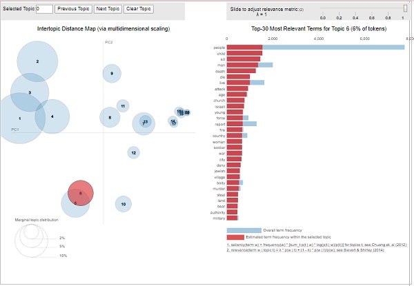
From the above output, the bubbles on the left-side represents a topic and larger the bubble, the more prevalent is that topic. The topic model will be good if the topic model has big, non-overlapping bubbles scattered throughout the chart.
Gensim - Creating LDA Mallet Model
This chapter will explain what is a Latent Dirichlet Allocation (LDA) Mallet Model and how to create the same in Gensim.
In the previous section we have implemented LDA model and get the topics from documents of 20Newsgroup dataset. That was Gensims inbuilt version of the LDA algorithm. There is a Mallet version of Gensim also, which provides better quality of topics. Here, we are going to apply Mallets LDA on the previous example we have already implemented.
What is LDA Mallet Model?
Mallet, an open source toolkit, was written by Andrew McCullum. It is basically a Java based package which is used for NLP, document classification, clustering, topic modeling, and many other machine learning applications to text. It provides us the Mallet Topic Modeling toolkit which contains efficient, sampling-based implementations of LDA as well as Hierarchical LDA.
Mallet2.0 is the current release from MALLET, the java topic modeling toolkit. Before we start using it with Gensim for LDA, we must download the mallet-2.0.8.zip package on our system and unzip it. Once installed and unzipped, set the environment variable %MALLET_HOME% to the point to the MALLET directory either manually or by the code we will be providing, while implementing the LDA with Mallet next.
Gensim Wrapper
Python provides Gensim wrapper for Latent Dirichlet Allocation (LDA). The syntax of that wrapper is gensim.models.wrappers.LdaMallet. This module, collapsed gibbs sampling from MALLET, allows LDA model estimation from a training corpus and inference of topic distribution on new, unseen documents as well.
Implementation Example
We will be using LDA Mallet on previously built LDA model and will check the difference in performance by calculating Coherence score.
Providing Path to Mallet File
Before applying Mallet LDA model on our corpus built in previous example, we must have to update the environment variables and provide the path the Mallet file as well. It can be done with the help of following code −
import os
from gensim.models.wrappers import LdaMallet
os.environ.update({'MALLET_HOME':r'C:/mallet-2.0.8/'})
#You should update this path as per the path of Mallet directory on your system.
mallet_path = r'C:/mallet-2.0.8/bin/mallet'
#You should update this path as per the path of Mallet directory on your system.
Once we provided the path to Mallet file, we can now use it on the corpus. It can be done with the help of ldamallet.show_topics() function as follows −
ldamallet = gensim.models.wrappers.LdaMallet(
   mallet_path, corpus=corpus, num_topics=20, id2word=id2word
)
pprint(ldamallet.show_topics(formatted=False))
Output
[
   (4,
   [('gun', 0.024546225966016102),
   ('law', 0.02181426826996709),
   ('state', 0.017633545129043606),
   ('people', 0.017612848479831116),
   ('case', 0.011341763768445888),
   ('crime', 0.010596684396796159),
   ('weapon', 0.00985160502514643),
   ('person', 0.008671896020034356),
   ('firearm', 0.00838214293105946),
   ('police', 0.008257963035784506)]),
   (9,
   [('make', 0.02147966482730431),
   ('people', 0.021377478029838543),
   ('work', 0.018557122419783363),
   ('money', 0.016676885346413244),
   ('year', 0.015982015123646026),
   ('job', 0.012221540976905783),
   ('pay', 0.010239117106069897),
   ('time', 0.008910688739014919),
   ('school', 0.0079092581238504),
   ('support', 0.007357449417535254)]),
   (14,
   [('power', 0.018428398507941996),
   ('line', 0.013784244460364121),
   ('high', 0.01183271164249895),
   ('work', 0.011560979224821522),
   ('ground', 0.010770484918850819),
   ('current', 0.010745781971789235),
   ('wire', 0.008399002000938712),
   ('low', 0.008053160742076529),
   ('water', 0.006966231071366814),
   ('run', 0.006892122230182061)]),
   (0,
   [('people', 0.025218349201353372),
   ('kill', 0.01500904870564167),
   ('child', 0.013612400660948935),
   ('armenian', 0.010307655991816822),
   ('woman', 0.010287984892595798),
   ('start', 0.01003226060272248),
   ('day', 0.00967818081674404),
   ('happen', 0.009383114328428673),
   ('leave', 0.009383114328428673),
   ('fire', 0.009009363443229208)]),
   (1,
   [('file', 0.030686386604212003),
   ('program', 0.02227713642901929),
   ('window', 0.01945561169918489),
   ('set', 0.015914874783314277),
   ('line', 0.013831003577619592),
   ('display', 0.013794120901412606),
   ('application', 0.012576992586582082),
   ('entry', 0.009275993066056873),
   ('change', 0.00872275292295209),
   ('color', 0.008612104894331132)]),
   (12,
   [('line', 0.07153810971508515),
   ('buy', 0.02975597944523662),
   ('organization', 0.026877236406682988),
   ('host', 0.025451316957679788),
   ('price', 0.025182275552207485),
   ('sell', 0.02461728860071565),
   ('mail', 0.02192687454599263),
   ('good', 0.018967419085797303),
   ('sale', 0.017998870026097017),
   ('send', 0.013694207538540181)]),
   (11,
   [('thing', 0.04901329901329901),
   ('good', 0.0376018876018876),
   ('make', 0.03393393393393394),
   ('time', 0.03326898326898327),
   ('bad', 0.02664092664092664),
   ('happen', 0.017696267696267698),
   ('hear', 0.015615615615615615),
   ('problem', 0.015465465465465466),
   ('back', 0.015143715143715144),
   ('lot', 0.01495066495066495)]),
   (18,
   [('space', 0.020626317374284855),
   ('launch', 0.00965716006366413),
   ('system', 0.008560244332602057),
   ('project', 0.008173097603991913),
   ('time', 0.008108573149223556),
   ('cost', 0.007764442723792318),
   ('year', 0.0076784101174345075),
   ('earth', 0.007484836753129436),
   ('base', 0.0067535595990880545),
   ('large', 0.006689035144319697)]),
   (5,
   [('government', 0.01918437232469453),
   ('people', 0.01461203206475212),
   ('state', 0.011207097828624796),
   ('country', 0.010214802708381975),
   ('israeli', 0.010039691804809714),
   ('war', 0.009436532025838587),
   ('force', 0.00858043427504086),
   ('attack', 0.008424780138532182),
   ('land', 0.0076659662230523775),
   ('world', 0.0075103120865437)]),
   (2,
   [('car', 0.041091194044470564),
   ('bike', 0.015598981291017729),
   ('ride', 0.011019688510138114),
   ('drive', 0.010627877363110981),
   ('engine', 0.009403467528651191),
   ('speed', 0.008081104907434616),
   ('turn', 0.007738270153785875),
   ('back', 0.007738270153785875),
   ('front', 0.007468899990204721),
   ('big', 0.007370947203447938)])
]
Evaluating Performance
Now we can also evaluate its performance by calculating the coherence score as follows −
ldamallet = gensim.models.wrappers.LdaMallet(
   mallet_path, corpus=corpus, num_topics=20, id2word=id2word
)
pprint(ldamallet.show_topics(formatted=False))
Output
Coherence Score: 0.5842762900901401
Gensim - Documents & LDA Model
This chapter discusses the documents and LDA model in Gensim.
Finding Optimal Number of Topics for LDA
We can find the optimal number of topics for LDA by creating many LDA models with various values of topics. Among those LDAs we can pick one having highest coherence value.
Following function named coherence_values_computation() will train multiple LDA models. It will also provide the models as well as their corresponding coherence score −
def coherence_values_computation(dictionary, corpus, texts, limit, start=2, step=3):
   coherence_values = []
   model_list = []
   for num_topics in range(start, limit, step):
      model = gensim.models.wrappers.LdaMallet(
         mallet_path, corpus=corpus, num_topics=num_topics, id2word=id2word
      )
      model_list.append(model)
   coherencemodel = CoherenceModel(
      model=model, texts=texts, dictionary=dictionary, coherence='c_v'
   )
   coherence_values.append(coherencemodel.get_coherence())
return model_list, coherence_values
Now with the help of following code, we can get the optimal number of topics which we can show with the help of a graph as well −
model_list, coherence_values = coherence_values_computation (
   dictionary=id2word, corpus=corpus, texts=data_lemmatized,
   start=1, limit=50, step=8
)
limit=50; start=1; step=8;
x = range(start, limit, step)
plt.plot(x, coherence_values)
plt.xlabel("Num Topics")
plt.ylabel("Coherence score")
plt.legend(("coherence_values"), loc='best')
plt.show()
Output
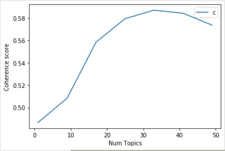
Next, we can also print the coherence values for various topics as follows −
for m, cv in zip(x, coherence_values):
   print("Num Topics =", m, " is having Coherence Value of", round(cv, 4))
Output
Num Topics = 1 is having Coherence Value of 0.4866
Num Topics = 9 is having Coherence Value of 0.5083
Num Topics = 17 is having Coherence Value of 0.5584
Num Topics = 25 is having Coherence Value of 0.5793
Num Topics = 33 is having Coherence Value of 0.587
Num Topics = 41 is having Coherence Value of 0.5842
Num Topics = 49 is having Coherence Value of 0.5735
Now, the question arises which model should we pick now? One of the good practices is to pick the model, that is giving highest coherence value before flattering out. So thats why, we will be choosing the model with 25 topics which is at number 4 in the above list.
optimal_model = model_list[3]
model_topics = optimal_model.show_topics(formatted=False)
pprint(optimal_model.print_topics(num_words=10))

[
   (0,
   '0.018*"power" + 0.011*"high" + 0.010*"ground" + 0.009*"current" + '
   '0.008*"low" + 0.008*"wire" + 0.007*"water" + 0.007*"work" + 0.007*"design" '
   '+ 0.007*"light"'),
   (1,
   '0.036*"game" + 0.029*"team" + 0.029*"year" + 0.028*"play" + 0.020*"player" '
   '+ 0.019*"win" + 0.018*"good" + 0.013*"season" + 0.012*"run" + 0.011*"hit"'),
   (2,
   '0.020*"image" + 0.019*"information" + 0.017*"include" + 0.017*"mail" + '
   '0.016*"send" + 0.015*"list" + 0.013*"post" + 0.012*"address" + '
   '0.012*"internet" + 0.012*"system"'),
   (3,
   '0.986*"ax" + 0.002*"_" + 0.001*"tm" + 0.000*"part" + 0.000*"biz" + '
   '0.000*"mb" + 0.000*"mbs" + 0.000*"pne" + 0.000*"end" + 0.000*"di"'),
   (4,
   '0.020*"make" + 0.014*"work" + 0.013*"money" + 0.013*"year" + 0.012*"people" '
   '+ 0.011*"job" + 0.010*"group" + 0.009*"government" + 0.008*"support" + '
   '0.008*"question"'),
   (5,
   '0.011*"study" + 0.011*"drug" + 0.009*"science" + 0.008*"food" + '
   '0.008*"problem" + 0.008*"result" + 0.008*"effect" + 0.007*"doctor" + '
   '0.007*"research" + 0.007*"patient"'),
   (6,
   '0.024*"gun" + 0.024*"law" + 0.019*"state" + 0.015*"case" + 0.013*"people" + '
   '0.010*"crime" + 0.010*"weapon" + 0.010*"person" + 0.008*"firearm" + '
   '0.008*"police"'),
   (7,
   '0.012*"word" + 0.011*"question" + 0.011*"exist" + 0.011*"true" + '
   '0.010*"religion" + 0.010*"claim" + 0.008*"argument" + 0.008*"truth" + '
   '0.008*"life" + 0.008*"faith"'),
   (8,
   '0.077*"time" + 0.029*"day" + 0.029*"call" + 0.025*"back" + 0.021*"work" + '
   '0.019*"long" + 0.015*"end" + 0.015*"give" + 0.014*"year" + 0.014*"week"'),
   (9,
   '0.048*"thing" + 0.041*"make" + 0.038*"good" + 0.037*"people" + '
   '0.028*"write" + 0.019*"bad" + 0.019*"point" + 0.018*"read" + 0.018*"post" + '
   '0.016*"idea"'),
   (10,
   '0.022*"book" + 0.020*"_" + 0.013*"man" + 0.012*"people" + 0.011*"write" + '
   '0.011*"find" + 0.010*"history" + 0.010*"armenian" + 0.009*"turkish" + '
   '0.009*"number"'),
   (11,
   '0.064*"line" + 0.030*"buy" + 0.028*"organization" + 0.025*"price" + '
   '0.025*"sell" + 0.023*"good" + 0.021*"host" + 0.018*"sale" + 0.017*"mail" + '
   '0.016*"cost"'),
   (12,
   '0.041*"car" + 0.015*"bike" + 0.011*"ride" + 0.010*"engine" + 0.009*"drive" '
   '+ 0.008*"side" + 0.008*"article" + 0.007*"turn" + 0.007*"front" + '
   '0.007*"speed"'),
   (13,
   '0.018*"people" + 0.011*"attack" + 0.011*"state" + 0.011*"israeli" + '
   '0.010*"war" + 0.010*"country" + 0.010*"government" + 0.009*"live" + '
   '0.009*"give" + 0.009*"land"'),
   (14,
   '0.037*"file" + 0.026*"line" + 0.021*"read" + 0.019*"follow" + '
   '0.018*"number" + 0.015*"program" + 0.014*"write" + 0.012*"entry" + '
   '0.012*"give" + 0.011*"check"'),
   (15,
   '0.196*"write" + 0.172*"line" + 0.165*"article" + 0.117*"organization" + '
   '0.086*"host" + 0.030*"reply" + 0.010*"university" + 0.008*"hear" + '
   '0.007*"post" + 0.007*"news"'),
   (16,
   '0.021*"people" + 0.014*"happen" + 0.014*"child" + 0.012*"kill" + '
   '0.011*"start" + 0.011*"live" + 0.010*"fire" + 0.010*"leave" + 0.009*"hear" '
   '+ 0.009*"home"'),
   (17,
   '0.038*"key" + 0.018*"system" + 0.015*"space" + 0.015*"technology" + '
   '0.014*"encryption" + 0.010*"chip" + 0.010*"bit" + 0.009*"launch" + '
   '0.009*"public" + 0.009*"government"'),
   (18,
   '0.035*"drive" + 0.031*"system" + 0.027*"problem" + 0.027*"card" + '
   '0.020*"driver" + 0.017*"bit" + 0.017*"work" + 0.016*"disk" + '
   '0.014*"monitor" + 0.014*"machine"'),
   (19,
   '0.031*"window" + 0.020*"run" + 0.018*"color" + 0.018*"program" + '
   '0.017*"application" + 0.016*"display" + 0.015*"set" + 0.015*"version" + '
   '0.012*"screen" + 0.012*"problem"')
]
Finding dominant topics in sentences
Finding dominant topics in sentences is one of the most useful practical applications of topic modeling. It determines what topic a given document is about. Here, we will find that topic number which has the highest percentage contribution in that particular document. In order to aggregate the information in a table, we will be creating a function named dominant_topics() −
def dominant_topics(ldamodel=lda_model, corpus=corpus, texts=data):
   sent_topics_df = pd.DataFrame()
Next, we will get the main topics in every document −
for i, row in enumerate(ldamodel[corpus]):
   row = sorted(row, key=lambda x: (x[1]), reverse=True)
Next, we will get the Dominant topic, Perc Contribution and Keywords for every document −
for j, (topic_num, prop_topic) in enumerate(row):
   if j == 0: # => dominant topic
      wp = ldamodel.show_topic(topic_num)
      topic_keywords = ", ".join([word for word, prop in wp])
sent_topics_df = sent_topics_df.append(
   pd.Series([int(topic_num), round(prop_topic,4), topic_keywords]), ignore_index=True
)
   else:
      break
sent_topics_df.columns = ['Dominant_Topic', 'Perc_Contribution', 'Topic_Keywords']
With the help of following code, we will add the original text to the end of the output −
contents = pd.Series(texts)
   sent_topics_df = pd.concat([sent_topics_df, contents], axis=1)
   return(sent_topics_df)
df_topic_sents_keywords = dominant_topics(
   ldamodel=optimal_model, corpus=corpus, texts=data
)
Now, do the formatting of topics in the sentences as follows −
df_dominant_topic = df_topic_sents_keywords.reset_index()
df_dominant_topic.columns = [
   'Document_No', 'Dominant_Topic', 'Topic_Perc_Contrib', 'Keywords', 'Text'
]
Finally, we can show the dominant topics as follows −
df_dominant_topic.head(15)
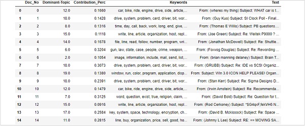
Finding Most Representative Document
In order to understand more about the topic, we can also find the documents, a given topic has contributed to the most. We can infer that topic by reading that particular document(s).
sent_topics_sorteddf_mallet = pd.DataFrame()
sent_topics_outdf_grpd = df_topic_sents_keywords.groupby('Dominant_Topic')
for i, grp in sent_topics_outdf_grpd:
   sent_topics_sorteddf_mallet = pd.concat([sent_topics_sorteddf_mallet,
grp.sort_values(['Perc_Contribution'], ascending=[0]).head(1)], axis=0)
sent_topics_sorteddf_mallet.reset_index(drop=True, inplace=True)
sent_topics_sorteddf_mallet.columns = [
   'Topic_Number', "Contribution_Perc", "Keywords", "Text"
]
sent_topics_sorteddf_mallet.head()
Output
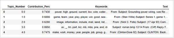
Volume & Distribution of Topics
Sometimes we also want to judge how widely the topic is discussed in documents. For this we need to understand the volume and distribution of topics across the documents.
First calculate the number of documents for every Topic as follows −
topic_counts = df_topic_sents_keywords['Dominant_Topic'].value_counts()
Next, calculate the percentage of Documents for every Topic as follows −;
topic_contribution = round(topic_counts/topic_counts.sum(), 4)
Now find the topic Number and Keywords as follows −
topic_num_keywords = df_topic_sents_keywords[['Dominant_Topic', 'Topic_Keywords']]
Now, concatenate then Column wise as follows −
df_dominant_topics = pd.concat(
   [topic_num_keywords, topic_counts, topic_contribution], axis=1
)
Next, we will change the Column names as follows −
df_dominant_topics.columns = [
   'Dominant-Topic', 'Topic-Keywords', 'Num_Documents', 'Perc_Documents'
]
df_dominant_topics
Output
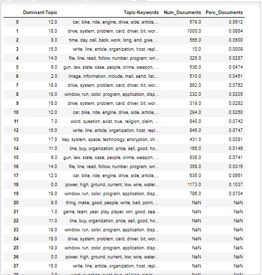
Gensim - Creating LSI & HDP Topic Model
This chapter deals with creating Latent Semantic Indexing (LSI) and Hierarchical Dirichlet Process (HDP) topic model with regards to Gensim.
The topic modeling algorithms that was first implemented in Gensim with Latent Dirichlet Allocation (LDA) is Latent Semantic Indexing (LSI). It is also called Latent Semantic Analysis (LSA). It got patented in 1988 by Scott Deerwester, Susan Dumais, George Furnas, Richard Harshman, Thomas Landaur, Karen Lochbaum, and Lynn Streeter.
In this section we are going to set up our LSI model. It can be done in the same way of setting up LDA model. We need to import LSI model from gensim.models.
Role of LSI
Actually, LSI is a technique NLP, especially in distributional semantics. It analyses the relationship between a set of documents and the terms these documents contain. If we talk about its working, then it constructs a matrix that contains word counts per document from a large piece of text.
Once constructed, to reduce the number of rows, LSI model use a mathematical technique called singular value decomposition (SVD). Along with reducing the number of rows, it also preserves the similarity structure among columns.
In matrix, the rows represent unique words and the columns represent each document. It works based on distributional hypothesis, i.e. it assumes that the words that are close in meaning will occur in same kind of text.
Implementation with Gensim
Here, we are going to use LSI (Latent Semantic Indexing) to extract the naturally discussed topics from dataset.
Loading Data Set
The dataset which we are going to use is the dataset of 20 Newsgroups having thousands of news articles from various sections of a news report. It is available under Sklearn data sets. We can easily download with the help of following Python script −
from sklearn.datasets import fetch_20newsgroups
newsgroups_train = fetch_20newsgroups(subset='train')
Lets look at some of the sample news with the help of following script −
newsgroups_train.data[:4]
["From: lerxst@wam.umd.edu (where's my thing)\nSubject:
WHAT car is this!?\nNntp-Posting-Host: rac3.wam.umd.edu\nOrganization:
University of Maryland, College Park\nLines: 15\n\n
I was wondering if anyone out there could enlighten me on this car
I saw\nthe other day. It was a 2-door sports car,
looked to be from the late 60s/\nearly 70s. It was called a Bricklin.
The doors were really small. In addition,\nthe front bumper was separate from
the rest of the body. This is \nall I know. If anyone can tellme a model name,
engine specs, years\nof production, where this car is made, history, or
whatever info you\nhave on this funky looking car,
please e-mail.\n\nThanks,\n- IL\n ---- brought to you by your neighborhood
Lerxst ----\n\n\n\n\n",

"From: guykuo@carson.u.washington.edu (Guy Kuo)\nSubject:
SI Clock Poll - Final Call\nSummary: Final call for SI clock reports\nKeywords:
SI,acceleration,clock,upgrade\nArticle-I.D.: shelley.1qvfo9INNc3s\nOrganization:
University of Washington\nLines: 11\nNNTP-Posting-Host: carson.u.washington.edu\n\nA
fair number of brave souls who upgraded their SI clock oscillator have\nshared their
experiences for this poll. Please send a brief message detailing\nyour experiences with
the procedure. Top speed attained, CPU rated speed,\nadd on cards and adapters, heat
sinks, hour of usage per day, floppy disk\nfunctionality with 800 and 1.4 m floppies
are especially requested.\n\nI will be summarizing in the next two days, so please add
to the network\nknowledge base if you have done the clock upgrade and haven't answered
this\npoll. Thanks.\n\nGuy Kuo <guykuo@u.washington.edu>\n",

'From: twillis@ec.ecn.purdue.edu (Thomas E Willis)\nSubject:
PB questions...\nOrganization: Purdue University Engineering Computer
Network\nDistribution: usa\nLines: 36\n\nwell folks, my mac plus finally gave up the
ghost this weekend after\nstarting life as a 512k way back in 1985. sooo, i\'m in the
market for a\nnew machine a bit sooner than i intended to be...\n\ni\'m looking into
picking up a powerbook 160 or maybe 180 and have a bunch\nof questions that (hopefully)
somebody can answer:\n\n* does anybody know any dirt on when the next round of
powerbook\nintroductions are expected? i\'d heard the 185c was supposed to make
an\nappearence "this summer" but haven\'t heard anymore on it - and since i\ndon\'t
have access to macleak, i was wondering if anybody out there had\nmore info...\n\n* has
anybody heard rumors about price drops to the powerbook line like the\nones the duo\'s
just went through recently?\n\n* what\'s the impression of the display on the 180? i
could probably swing\na 180 if i got the 80Mb disk rather than the 120, but i don\'t
really have\na feel for how much "better" the display is (yea, it looks great in
the\nstore, but is that all "wow" or is it really that good?). could i solicit\nsome
opinions of people who use the 160 and 180 day-to-day on if its worth\ntaking the disk
size and money hit to get the active display? (i realize\nthis is a real subjective
question, but i\'ve only played around with the\nmachines in a computer store breifly
and figured the opinions of somebody\nwho actually uses the machine daily might prove
helpful).\n\n* how well does hellcats perform? ;)\n\nthanks a bunch in advance for any
info - if you could email, i\'ll post a\nsummary (news reading time is at a premium
with finals just around the\ncorner... :( )\n--\nTom Willis \\ twillis@ecn.purdue.edu
\\ Purdue Electrical
Engineering\n---------------------------------------------------------------------------\
n"Convictions are more dangerous enemies of truth than lies." - F. W.\nNietzsche\n',

'From: jgreen@amber (Joe Green)\nSubject: Re: Weitek P9000 ?\nOrganization: Harris
Computer Systems Division\nLines: 14\nDistribution: world\nNNTP-Posting-Host:
amber.ssd.csd.harris.com\nX-Newsreader: TIN [version 1.1 PL9]\n\nRobert J.C. Kyanko
(rob@rjck.UUCP) wrote:\n > abraxis@iastate.edu writes in article <
abraxis.734340159@class1.iastate.edu>:\n> > Anyone know about the Weitek P9000
graphics chip?\n > As far as the low-level stuff goes, it looks pretty nice. It\'s
got this\n > quadrilateral fill command that requires just the four
points.\n\nDo you have Weitek\'s address/phone number? I\'d like to get some
information\nabout this chip.\n\n--\nJoe Green\t\t\t\tHarris
Corporation\njgreen@csd.harris.com\t\t\tComputer Systems Division\n"The only thing that
really scares me is a person with no sense of humor."\n\t\t\t\t\t\t-- Jonathan
Winters\n']
Prerequisite
We need Stopwords from NLTK and English model from Scapy. Both can be downloaded as follows −
import nltk;
nltk.download('stopwords')
nlp = spacy.load('en_core_web_md', disable=['parser', 'ner'])
Importing Necessary Packages
In order to build LSI model we need to import following necessary package −
import re
import numpy as np
import pandas as pd
from pprint import pprint
import gensim
import gensim.corpora as corpora
from gensim.utils import simple_preprocess
from gensim.models import CoherenceModel
import spacy
import matplotlib.pyplot as plt
Preparing Stopwords
Now we need to import the Stopwords and use them −
from nltk.corpus import stopwords
stop_words = stopwords.words('english')
stop_words.extend(['from', 'subject', 're', 'edu', 'use'])
Clean Up the Text
Now, with the help of Gensims simple_preprocess() we need to tokenise each sentence into a list of words. We should also remove the punctuations and unnecessary characters. In order to do this, we will create a function named sent_to_words() −
def sent_to_words(sentences):
   for sentence in sentences:
      yield(gensim.utils.simple_preprocess(str(sentence), deacc=True))
data_words = list(sent_to_words(data))
Building Bigram & Trigram Models
As we know that bigrams are two words that are frequently occurring together in the document and trigram are three words that are frequently occurring together in the document. With the help of Gensims Phrases model, we can do this −
bigram = gensim.models.Phrases(data_words, min_count=5, threshold=100)
trigram = gensim.models.Phrases(bigram[data_words], threshold=100)
bigram_mod = gensim.models.phrases.Phraser(bigram)
trigram_mod = gensim.models.phrases.Phraser(trigram)
Filter out Stopwords
Next, we need to filter out the Stopwords. Along with that, we will also create functions to make bigrams, trigrams and for lemmatisation −
def remove_stopwords(texts):
   return [[word for word in simple_preprocess(str(doc))
   if word not in stop_words] for doc in texts]
def make_bigrams(texts):
   return [bigram_mod[doc] for doc in texts]
def make_trigrams(texts):
   return [trigram_mod[bigram_mod[doc]] for doc in texts]
def lemmatization(texts, allowed_postags=['NOUN', 'ADJ', 'VERB', 'ADV']):
   texts_out = []
   for sent in texts:
      doc = nlp(" ".join(sent))
      texts_out.append([token.lemma_ for token in doc if token.pos_ in allowed_postags])
   return texts_out
Building Dictionary & Corpus for Topic Model
We now need to build the dictionary & corpus. We did it in the previous examples as well −
id2word = corpora.Dictionary(data_lemmatized)
texts = data_lemmatized
corpus = [id2word.doc2bow(text) for text in texts]
Building LSI Topic Model
We already implemented everything that is required to train the LSI model. Now, it is the time to build the LSI topic model. For our implementation example, it can be done with the help of following line of codes −
lsi_model = gensim.models.lsimodel.LsiModel(
   corpus=corpus, id2word=id2word, num_topics=20,chunksize=100
)
Implementation Example
Lets see the complete implementation example to build LDA topic model −
import re
import numpy as np
import pandas as pd
from pprint import pprint
import gensim
import gensim.corpora as corpora
from gensim.utils import simple_preprocess
from gensim.models import CoherenceModel
import spacy
import matplotlib.pyplot as plt
from nltk.corpus import stopwords
stop_words = stopwords.words('english')
stop_words.extend(['from', 'subject', 're', 'edu', 'use'])
from sklearn.datasets import fetch_20newsgroups
newsgroups_train = fetch_20newsgroups(subset='train')
data = newsgroups_train.data
data = [re.sub('\S*@\S*\s?', '', sent) for sent in data]
data = [re.sub('\s+', ' ', sent) for sent in data]
data = [re.sub("\'", "", sent) for sent in data]
print(data_words[:4]) #it will print the data after prepared for stopwords
bigram = gensim.models.Phrases(data_words, min_count=5, threshold=100)
trigram = gensim.models.Phrases(bigram[data_words], threshold=100)
bigram_mod = gensim.models.phrases.Phraser(bigram)
trigram_mod = gensim.models.phrases.Phraser(trigram)
def remove_stopwords(texts):
   return [[word for word in simple_preprocess(str(doc))
   if word not in stop_words] for doc in texts]
def make_bigrams(texts):
   return [bigram_mod[doc] for doc in texts]
def make_trigrams(texts):
   return [trigram_mod[bigram_mod[doc]] for doc in texts]
def lemmatization(texts, allowed_postags=['NOUN', 'ADJ', 'VERB', 'ADV']):
   texts_out = []
   for sent in texts:
      doc = nlp(" ".join(sent))
      texts_out.append([token.lemma_ for token in doc if token.pos_ in allowed_postags])
return texts_out
data_words_nostops = remove_stopwords(data_words)
data_words_bigrams = make_bigrams(data_words_nostops)
nlp = spacy.load('en_core_web_md', disable=['parser', 'ner'])
data_lemmatized = lemmatization(
   data_words_bigrams, allowed_postags=['NOUN', 'ADJ', 'VERB', 'ADV']
)
print(data_lemmatized[:4]) #it will print the lemmatized data.
id2word = corpora.Dictionary(data_lemmatized)
texts = data_lemmatized
corpus = [id2word.doc2bow(text) for text in texts]
print(corpus[:4]) #it will print the corpus we created above.
[[(id2word[id], freq) for id, freq in cp] for cp in corpus[:4]]
#it will print the words with their frequencies.
lsi_model = gensim.models.lsimodel.LsiModel(
   corpus=corpus, id2word=id2word, num_topics=20,chunksize=100
)
We can now use the above created LSI model to get the topics.
Viewing Topics in LSI Model
The LSI model (lsi_model) we have created above can be used to view the topics from the documents. It can be done with the help of following script −
pprint(lsi_model.print_topics())
doc_lsi = lsi_model[corpus]
Output
[
   (0,
   '1.000*"ax" + 0.001*"_" + 0.000*"tm" + 0.000*"part" +    0.000*"pne" + '
   '0.000*"biz" + 0.000*"mbs" + 0.000*"end" + 0.000*"fax" + 0.000*"mb"'),
   (1,
   '0.239*"say" + 0.222*"file" + 0.189*"go" + 0.171*"know" + 0.169*"people" + '
   '0.147*"make" + 0.140*"use" + 0.135*"also" + 0.133*"see" + 0.123*"think"')
]
Hierarchical Dirichlet Process (HPD)
Topic models such as LDA and LSI helps in summarising and organising large archives of texts that is not possible to analyse by hand. Apart from LDA and LSI, one other powerful topic model in Gensim is HDP (Hierarchical Dirichlet Process). Its basically a mixed-membership model for unsupervised analysis of grouped data. Unlike LDA (itss finite counterpart), HDP infers the number of topics from the data.
Implementation With Gensim
For implementing HDP in Gensim, we need to train corpus and dictionary (as did in the above examples while implementing LDA and LSI topic models) HDP topic model that we can import from gensim.models.HdpModel. Here also we will implement HDP topic model on 20Newsgroup data and the steps are also same.
For our corpus and dictionary (created in above examples for LSI and LDA model), we can import HdpModel as follows −
Hdp_model = gensim.models.hdpmodel.HdpModel(corpus=corpus, id2word=id2word)
Viewing Topics in LSI Model
The HDP model (Hdp_model) can be used to view the topics from the documents. It can be done with the help of following script −
pprint(Hdp_model.print_topics())
Output
[
   (0,
   '0.009*line + 0.009*write + 0.006*say + 0.006*article + 0.006*know + '
   '0.006*people + 0.005*make + 0.005*go + 0.005*think + 0.005*be'),
   (1,
   '0.016*line + 0.011*write + 0.008*article + 0.008*organization + 0.006*know '
   '+ 0.006*host + 0.006*be + 0.005*get + 0.005*use + 0.005*say'),
   (2,
   '0.810*ax + 0.001*_ + 0.000*tm + 0.000*part + 0.000*mb + 0.000*pne + '
   '0.000*biz + 0.000*end + 0.000*wwiz + 0.000*fax'),
   (3,
   '0.015*line + 0.008*write + 0.007*organization + 0.006*host + 0.006*know + '
   '0.006*article + 0.005*use + 0.005*thank + 0.004*get + 0.004*problem'),
   (4,
   '0.004*line + 0.003*write + 0.002*believe + 0.002*think + 0.002*article + '
   '0.002*belief + 0.002*say + 0.002*see + 0.002*look + 0.002*organization'),
   (5,
   '0.005*line + 0.003*write + 0.003*organization + 0.002*article + 0.002*time '
   '+ 0.002*host + 0.002*get + 0.002*look + 0.002*say + 0.001*number'),
   (6,
   '0.003*line + 0.002*say + 0.002*write + 0.002*go + 0.002*gun + 0.002*get + '
   '0.002*organization + 0.002*bill + 0.002*article + 0.002*state'),
   (7,
   '0.003*line + 0.002*write + 0.002*article + 0.002*organization + 0.001*none '
   '+ 0.001*know + 0.001*say + 0.001*people + 0.001*host + 0.001*new'),
   (8,
   '0.004*line + 0.002*write + 0.002*get + 0.002*team + 0.002*organization + '
   '0.002*go + 0.002*think + 0.002*know + 0.002*article + 0.001*well'),
   (9,
   '0.004*line + 0.002*organization + 0.002*write + 0.001*be + 0.001*host + '
   '0.001*article + 0.001*thank + 0.001*use + 0.001*work + 0.001*run'),
   (10,
   '0.002*line + 0.001*game + 0.001*write + 0.001*get + 0.001*know + '
   '0.001*thing + 0.001*think + 0.001*article + 0.001*help + 0.001*turn'),
   (11,
   '0.002*line + 0.001*write + 0.001*game + 0.001*organization + 0.001*say + '
   '0.001*host + 0.001*give + 0.001*run + 0.001*article + 0.001*get'),
   (12,
   '0.002*line + 0.001*write + 0.001*know + 0.001*time + 0.001*article + '
   '0.001*get + 0.001*think + 0.001*organization + 0.001*scope + 0.001*make'),
   (13,
   '0.002*line + 0.002*write + 0.001*article + 0.001*organization + 0.001*make '
   '+ 0.001*know + 0.001*see + 0.001*get + 0.001*host + 0.001*really'),
   (14,
   '0.002*write + 0.002*line + 0.002*know + 0.001*think + 0.001*say + '
   '0.001*article + 0.001*argument + 0.001*even + 0.001*card + 0.001*be'),
   (15,
   '0.001*article + 0.001*line + 0.001*make + 0.001*write + 0.001*know + '
   '0.001*say + 0.001*exist + 0.001*get + 0.001*purpose + 0.001*organization'),
   (16,
   '0.002*line + 0.001*write + 0.001*article + 0.001*insurance + 0.001*go + '
   '0.001*be + 0.001*host + 0.001*say + 0.001*organization + 0.001*part'),
   (17,
   '0.001*line + 0.001*get + 0.001*hit + 0.001*go + 0.001*write + 0.001*say + '
   '0.001*know + 0.001*drug + 0.001*see + 0.001*need'),
   (18,
   '0.002*option + 0.001*line + 0.001*flight + 0.001*power + 0.001*software + '
   '0.001*write + 0.001*add + 0.001*people + 0.001*organization + 0.001*module'),
   (19,
   '0.001*shuttle + 0.001*line + 0.001*roll + 0.001*attitude + 0.001*maneuver + '
   '0.001*mission + 0.001*also + 0.001*orbit + 0.001*produce + 0.001*frequency')
]
Gensim - Developing Word Embedding
The chapter will help us understand developing word embedding in Gensim.
Word embedding, approach to represent words & document, is a dense vector representation for text where words having the same meaning have a similar representation. Following are some characteristics of word embedding −
It is a class of technique which represents the individual words as real-valued vectors in a pre-defined vector space.
This technique is often lumped into the field of DL (deep learning) because every word is mapped to one vector and the vector values are learned in the same way a NN (Neural Networks) does.
The key approach of word embedding technique is a dense distributed representation for every word.
Different Word Embedding Methods/Algorithms
As discussed above, word embedding methods/algorithms learn a real-valued vector representation from a corpus of text. This learning process can either use with the NN model on task like document classification or is an unsupervised process such as document statistics. Here we are going to discuss two methods/algorithm that can be used to learn a word embedding from text −
Word2Vec by Google
Word2Vec, developed by Tomas Mikolov, et. al. at Google in 2013, is a statistical method for efficiently learning a word embedding from text corpus. Its actually developed as a response to make NN based training of word embedding more efficient. It has become the de facto standard for word embedding.
Word embedding by Word2Vec involves analysis of the learned vectors as well as exploration of vector math on representation of words. Following are the two different learning methods which can be used as the part of Word2Vec method −
- CBoW(Continuous Bag of Words) Model
- Continuous Skip-Gram Model
GloVe by Standford
GloVe(Global vectors for Word Representation), is an extension to the Word2Vec method. It was developed by Pennington et al. at Stanford. GloVe algorithm is a mix of both −
- Global statistics of matrix factorization techniques like LSA (Latent Semantic Analysis)
- Local context-based learning in Word2Vec.
If we talk about its working then instead of using a window to define local context, GloVe constructs an explicit word co-occurrence matrix using statistics across the whole text corpus.
Developing Word2Vec Embedding
Here, we will develop Word2Vec embedding by using Gensim. In order to work with a Word2Vec model, Gensim provides us Word2Vec class which can be imported from models.word2vec. For its implementation, word2vec requires a lot of text e.g. the entire Amazon review corpus. But here, we will apply this principle on small-in memory text.
Implementation Example
First we need to import the Word2Vec class from gensim.models as follows −
from gensim.models import Word2Vec
Next, we need to define the training data. Rather than taking big text file, we are using some sentences to implement this principal.
sentences = [
   ['this', 'is', 'gensim', 'tutorial', 'for', 'free'],
   ['this', 'is', 'the', 'tutorials' 'point', 'website'],
   ['you', 'can', 'read', 'technical','tutorials', 'for','free'],
   ['we', 'are', 'implementing','word2vec'],
   ['learn', 'full', 'gensim', 'tutorial']
]
Once the training data is provided, we need to train the model. it can be done as follows −
model = Word2Vec(sentences, min_count=1)
We can summarise the model as follows −;
print(model)
We can summarise the vocabulary as follows −
words = list(model.wv.vocab)
print(words)
Next, lets access the vector for one word. We are doing it for the word tutorial.
print(model['tutorial'])
Next, we need to save the model −
model.save('model.bin')
Next, we need to load the model −
new_model = Word2Vec.load('model.bin')
Finally, print the saved model as follows −
print(new_model)
Complete Implementation Example
from gensim.models import Word2Vec
sentences = [
   ['this', 'is', 'gensim', 'tutorial', 'for', 'free'],
   ['this', 'is', 'the', 'tutorials' 'point', 'website'],
   ['you', 'can', 'read', 'technical','tutorials', 'for','free'],
   ['we', 'are', 'implementing','word2vec'],
   ['learn', 'full', 'gensim', 'tutorial']
]
model = Word2Vec(sentences, min_count=1)
print(model)
words = list(model.wv.vocab)
print(words)
print(model['tutorial'])
model.save('model.bin')
new_model = Word2Vec.load('model.bin')
print(new_model)
Output
Word2Vec(vocab=20, size=100, alpha=0.025)
[
   'this', 'is', 'gensim', 'tutorial', 'for', 'free', 'the', 'tutorialspoint',
   'website', 'you', 'can', 'read', 'technical', 'tutorials', 'we', 'are',
   'implementing', 'word2vec', 'learn', 'full'
]
[
   -2.5256255e-03 -4.5352755e-03 3.9024993e-03 -4.9509313e-03
   -1.4255195e-03 -4.0217536e-03 4.9407515e-03 -3.5925603e-03
   -1.1933431e-03 -4.6682903e-03 1.5440651e-03 -1.4101702e-03
   3.5070938e-03 1.0914479e-03 2.3334436e-03 2.4452661e-03
   -2.5336299e-04 -3.9676363e-03 -8.5054158e-04 1.6443320e-03
   -4.9968651e-03 1.0974540e-03 -1.1123562e-03 1.5393364e-03
   9.8941079e-04 -1.2656028e-03 -4.4471184e-03 1.8309267e-03
   4.9302122e-03 -1.0032534e-03 4.6892050e-03 2.9563988e-03
   1.8730218e-03 1.5343715e-03 -1.2685956e-03 8.3664013e-04
   4.1721235e-03 1.9445885e-03 2.4097660e-03 3.7517555e-03
   4.9687522e-03 -1.3598346e-03 7.1032363e-04 -3.6595813e-03
   6.0000515e-04 3.0872561e-03 -3.2115565e-03 3.2270295e-03
   -2.6354722e-03 -3.4988276e-04 1.8574356e-04 -3.5757164e-03
   7.5391348e-04 -3.5205986e-03 -1.9795434e-03 -2.8321696e-03
   4.7155009e-03 -4.3349937e-04 -1.5320212e-03 2.7013756e-03
   -3.7055744e-03 -4.1658725e-03 4.8034848e-03 4.8594419e-03
   3.7129463e-03 4.2385766e-03 2.4612297e-03 5.4920948e-04
   -3.8912550e-03 -4.8226118e-03 -2.2763973e-04 4.5571579e-03
   -3.4609400e-03 2.7903817e-03 -3.2709218e-03 -1.1036445e-03
   2.1492650e-03 -3.0384419e-04 1.7709908e-03 1.8429896e-03
   -3.4038599e-03 -2.4872608e-03 2.7693063e-03 -1.6352943e-03
   1.9182395e-03 3.7772327e-03 2.2769428e-03 -4.4629495e-03
   3.3151123e-03 4.6509290e-03 -4.8521687e-03 6.7615538e-04
   3.1034781e-03 2.6369948e-05 4.1454583e-03 -3.6932561e-03
   -1.8769916e-03 -2.1958587e-04 6.3395966e-04 -2.4969708e-03
]
Word2Vec(vocab=20, size=100, alpha=0.025)
Visualising Word Embedding
We can also explore the word embedding with visualisation. It can be done by using a classical projection method (like PCA) to reduce the high-dimensional word vectors to 2-D plots. Once reduced, we can then plot them on graph.
Plotting Word Vectors Using PCA
First, we need to retrieve all the vectors from a trained model as follows −
Z = model[model.wv.vocab]
Next, we need to create a 2-D PCA model of word vectors by using PCA class as follows −
pca = PCA(n_components=2)
result = pca.fit_transform(Z)
Now, we can plot the resulting projection by using the matplotlib as follows −
Pyplot.scatter(result[:,0],result[:,1])
We can also annotate the points on the graph with the words itself. Plot the resulting projection by using the matplotlib as follows −
words = list(model.wv.vocab)
for i, word in enumerate(words):
   pyplot.annotate(word, xy=(result[i, 0], result[i, 1]))
Complete Implementation Example
from gensim.models import Word2Vec
from sklearn.decomposition import PCA
from matplotlib import pyplot
sentences = [
   ['this', 'is', 'gensim', 'tutorial', 'for', 'free'],
	['this', 'is', 'the', 'tutorials' 'point', 'website'],
	['you', 'can', 'read', 'technical','tutorials', 'for','free'],
	['we', 'are', 'implementing','word2vec'],
	['learn', 'full', 'gensim', 'tutorial']
]
model = Word2Vec(sentences, min_count=1)
X = model[model.wv.vocab]
pca = PCA(n_components=2)
result = pca.fit_transform(X)
pyplot.scatter(result[:, 0], result[:, 1])
words = list(model.wv.vocab)
for i, word in enumerate(words):
   pyplot.annotate(word, xy=(result[i, 0], result[i, 1]))
pyplot.show()
Output
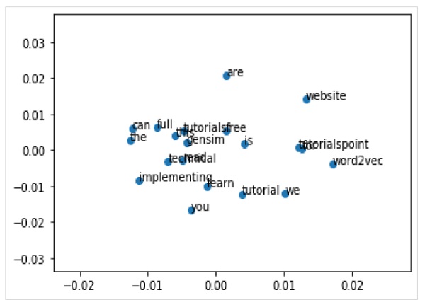
Gensim - Doc2Vec Model
Doc2Vec model, as opposite to Word2Vec model, is used to create a vectorised representation of a group of words taken collectively as a single unit. It doesnt only give the simple average of the words in the sentence.
Creating Document Vectors Using Doc2Vec
Here to create document vectors using Doc2Vec, we will be using text8 dataset which can be downloaded from gensim.downloader.
Downloading the Dataset
We can download the text8 dataset by using the following commands −
import gensim
import gensim.downloader as api
dataset = api.load("text8")
data = [d for d in dataset]
It will take some time to download the text8 dataset.
Train the Doc2Vec
In order to train the model, we need the tagged document which can be created by using models.doc2vec.TaggedDcument() as follows −
def tagged_document(list_of_list_of_words):
   for i, list_of_words in enumerate(list_of_list_of_words):
      yield gensim.models.doc2vec.TaggedDocument(list_of_words, [i])
data_for_training = list(tagged_document(data))
We can print the trained dataset as follows −
print(data_for_training [:1])
Output
[TaggedDocument(words=['anarchism', 'originated', 'as', 'a', 'term', 'of',
'abuse', 'first', 'used', 'against', 'early', 'working', 'class', 'radicals',
'including', 'the', 'diggers', 'of', 'the', 'english', 'revolution',
'and', 'the', 'sans', 'culottes', 'of', 'the', 'french', 'revolution',
'whilst', 'the', 'term', 'is', 'still', 'used', 'in', 'a', 'pejorative',
'way', 'to', 'describe', 'any', 'act', 'that', 'used', 'violent',
'means', 'to', 'destroy',
'the', 'organization', 'of', 'society', 'it', 'has', 'also', 'been'
, 'taken', 'up', 'as', 'a', 'positive', 'label', 'by', 'self', 'defined',
'anarchists', 'the', 'word', 'anarchism', 'is', 'derived', 'from', 'the',
'greek', 'without', 'archons', 'ruler', 'chief', 'king', 'anarchism',
'as', 'a', 'political', 'philosophy', 'is', 'the', 'belief', 'that',
'rulers', 'are', 'unnecessary', 'and', 'should', 'be', 'abolished',
'although', 'there', 'are', 'differing', 'interpretations', 'of',
'what', 'this', 'means', 'anarchism', 'also', 'refers', 'to',
'related', 'social', 'movements', 'that', 'advocate', 'the',
'elimination', 'of', 'authoritarian', 'institutions', 'particularly',
'the', 'state', 'the', 'word', 'anarchy', 'as', 'most', 'anarchists',
'use', 'it', 'does', 'not', 'imply', 'chaos', 'nihilism', 'or', 'anomie',
'but', 'rather', 'a', 'harmonious', 'anti', 'authoritarian', 'society',
'in', 'place', 'of', 'what', 'are', 'regarded', 'as', 'authoritarian',
'political', 'structures', 'and', 'coercive', 'economic', 'institutions',
'anarchists', 'advocate', 'social', 'relations', 'based', 'upon', 'voluntary',
'association', 'of', 'autonomous', 'individuals', 'mutual', 'aid', 'and',
'self', 'governance', 'while', 'anarchism', 'is', 'most', 'easily', 'defined',
'by', 'what', 'it', 'is', 'against', 'anarchists', 'also', 'offer',
'positive', 'visions', 'of', 'what', 'they', 'believe', 'to', 'be', 'a',
'truly', 'free', 'society', 'however', 'ideas', 'about', 'how', 'an', 'anarchist',
'society', 'might', 'work', 'vary', 'considerably', 'especially', 'with',
'respect', 'to', 'economics', 'there', 'is', 'also', 'disagreement', 'about',
'how', 'a', 'free', 'society', 'might', 'be', 'brought', 'about', 'origins',
'and', 'predecessors', 'kropotkin', 'and', 'others', 'argue', 'that', 'before',
'recorded', 'history', 'human', 'society', 'was', 'organized', 'on', 'anarchist',
'principles', 'most', 'anthropologists', 'follow', 'kropotkin', 'and', 'engels',
'in', 'believing', 'that', 'hunter', 'gatherer', 'bands', 'were', 'egalitarian',
'and', 'lacked', 'division', 'of', 'labour', 'accumulated', 'wealth', 'or', 'decreed',
'law', 'and', 'had', 'equal', 'access', 'to', 'resources', 'william', 'godwin',
'anarchists', 'including', 'the', 'the', 'anarchy', 'organisation', 'and', 'rothbard',
'find', 'anarchist', 'attitudes', 'in', 'taoism', 'from', 'ancient', 'china',
'kropotkin', 'found', 'similar', 'ideas', 'in', 'stoic', 'zeno', 'of', 'citium',
'according', 'to', 'kropotkin', 'zeno', 'repudiated', 'the', 'omnipotence', 'of',
'the', 'state', 'its', 'intervention', 'and', 'regimentation', 'and', 'proclaimed',
'the', 'sovereignty', 'of', 'the', 'moral', 'law', 'of', 'the', 'individual', 'the',
'anabaptists', 'of', 'one', 'six', 'th', 'century', 'europe', 'are', 'sometimes',
'considered', 'to', 'be', 'religious', 'forerunners', 'of', 'modern', 'anarchism',
'bertrand', 'russell', 'in', 'his', 'history', 'of', 'western', 'philosophy',
'writes', 'that', 'the', 'anabaptists', 'repudiated', 'all', 'law', 'since',
'they', 'held', 'that', 'the', 'good', 'man', 'will', 'be', 'guided', 'at',
'every', 'moment', 'by', 'the', 'holy', 'spirit', 'from', 'this', 'premise',
'they', 'arrive', 'at', 'communism', 'the', 'diggers', 'or', 'true', 'levellers',
'were', 'an', 'early', 'communistic', 'movement',
(truncated)
Initialise the Model
Once trained we now need to initialise the model. it can be done as follows −
model = gensim.models.doc2vec.Doc2Vec(vector_size=40, min_count=2, epochs=30)
Now, build the vocabulary as follows −
model.build_vocab(data_for_training)
Now, lets train the Doc2Vec model as follows −
model.train(data_for_training, total_examples=model.corpus_count, epochs=model.epochs)
Analysing the Output
Finally, we can analyse the output by using model.infer_vector() as follows −
print(model.infer_vector(['violent', 'means', 'to', 'destroy', 'the','organization']))
Complete Implementation Example
import gensim
import gensim.downloader as api
dataset = api.load("text8")
data = [d for d in dataset]
def tagged_document(list_of_list_of_words):
   for i, list_of_words in enumerate(list_of_list_of_words):
      yield gensim.models.doc2vec.TaggedDocument(list_of_words, [i])
data_for_training = list(tagged_document(data))
print(data_for_training[:1])
model = gensim.models.doc2vec.Doc2Vec(vector_size=40, min_count=2, epochs=30)
model.build_vocab(data_training)
model.train(data_training, total_examples=model.corpus_count, epochs=model.epochs)
print(model.infer_vector(['violent', 'means', 'to', 'destroy', 'the','organization']))
Output
[
   -0.2556166 0.4829361 0.17081228 0.10879577 0.12525807 0.10077011
   -0.21383236 0.19294572 0.11864349 -0.03227958 -0.02207291 -0.7108424
   0.07165232 0.24221905 -0.2924459 -0.03543589 0.21840079 -0.1274817
   0.05455418 -0.28968817 -0.29146606 0.32885507 0.14689675 -0.06913587
   -0.35173815 0.09340707 -0.3803535 -0.04030455 -0.10004586 0.22192696
   0.2384828 -0.29779273 0.19236489 -0.25727913 0.09140676 0.01265439
   0.08077634 -0.06902497 -0.07175519 -0.22583418 -0.21653089 0.00347822
   -0.34096122 -0.06176808 0.22885063 -0.37295452 -0.08222228 -0.03148199
   -0.06487323 0.11387568
]
