- Genetic Algorithms – Home
- Genetic Algorithms – Introduction
- Genetic Algorithms – Fundamentals
- Genotype Representation
- Genetic Algorithms – Population
- Genetic Algorithms – Fitness Function
- Genetic Algorithms – Parent Selection
- Genetic Algorithms – Crossover
- Genetic Algorithms – Mutation
- Survivor Selection
- Termination Condition
- Models Of Lifetime Adaptation
- Effective Implementation
- Advanced Topics
- Application Areas
- Further Readings
Genetic Algorithms - Quick Guide
Genetic Algorithms - Introduction
Genetic Algorithm (GA) is a search-based optimization technique based on the principles of Genetics and Natural Selection. It is frequently used to find optimal or near-optimal solutions to difficult problems which otherwise would take a lifetime to solve. It is frequently used to solve optimization problems, in research, and in machine learning.
Introduction to Optimization
Optimization is the process of making something better. In any process, we have a set of inputs and a set of outputs as shown in the following figure.
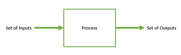
Optimization refers to finding the values of inputs in such a way that we get the best output values. The definition of best varies from problem to problem, but in mathematical terms, it refers to maximizing or minimizing one or more objective functions, by varying the input parameters.
The set of all possible solutions or values which the inputs can take make up the search space. In this search space, lies a point or a set of points which gives the optimal solution. The aim of optimization is to find that point or set of points in the search space.
What are Genetic Algorithms?
Nature has always been a great source of inspiration to all mankind. Genetic Algorithms (GAs) are search based algorithms based on the concepts of natural selection and genetics. GAs are a subset of a much larger branch of computation known as Evolutionary Computation.
GAs were developed by John Holland and his students and colleagues at the University of Michigan, most notably David E. Goldberg and has since been tried on various optimization problems with a high degree of success.
In GAs, we have a pool or a population of possible solutions to the given problem. These solutions then undergo recombination and mutation (like in natural genetics), producing new children, and the process is repeated over various generations. Each individual (or candidate solution) is assigned a fitness value (based on its objective function value) and the fitter individuals are given a higher chance to mate and yield more fitter individuals. This is in line with the Darwinian Theory of Survival of the Fittest.
In this way we keep evolving better individuals or solutions over generations, till we reach a stopping criterion.
Genetic Algorithms are sufficiently randomized in nature, but they perform much better than random local search (in which we just try various random solutions, keeping track of the best so far), as they exploit historical information as well.
Advantages of GAs
GAs have various advantages which have made them immensely popular. These include −
Does not require any derivative information (which may not be available for many real-world problems).
Is faster and more efficient as compared to the traditional methods.
Has very good parallel capabilities.
Optimizes both continuous and discrete functions and also multi-objective problems.
Provides a list of good solutions and not just a single solution.
Always gets an answer to the problem, which gets better over the time.
Useful when the search space is very large and there are a large number of parameters involved.
Limitations of GAs
Like any technique, GAs also suffer from a few limitations. These include −
GAs are not suited for all problems, especially problems which are simple and for which derivative information is available.
Fitness value is calculated repeatedly which might be computationally expensive for some problems.
Being stochastic, there are no guarantees on the optimality or the quality of the solution.
If not implemented properly, the GA may not converge to the optimal solution.
GA Motivation
Genetic Algorithms have the ability to deliver a good-enough solution fast-enough. This makes genetic algorithms attractive for use in solving optimization problems. The reasons why GAs are needed are as follows −
Solving Difficult Problems
In computer science, there is a large set of problems, which are NP-Hard. What this essentially means is that, even the most powerful computing systems take a very long time (even years!) to solve that problem. In such a scenario, GAs prove to be an efficient tool to provide usable near-optimal solutions in a short amount of time.
Failure of Gradient Based Methods
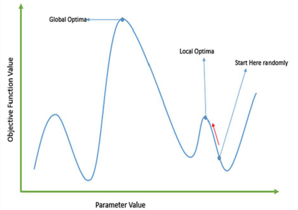
Traditional calculus based methods work by starting at a random point and by moving in the direction of the gradient, till we reach the top of the hill. This technique is efficient and works very well for single-peaked objective functions like the cost function in linear regression. But, in most real-world situations, we have a very complex problem called as landscapes, which are made of many peaks and many valleys, which causes such methods to fail, as they suffer from an inherent tendency of getting stuck at the local optima as shown in the following figure.
Getting a Good Solution Fast
Some difficult problems like the Travelling Salesperson Problem (TSP), have real-world applications like path finding and VLSI Design. Now imagine that you are using your GPS Navigation system, and it takes a few minutes (or even a few hours) to compute the optimal path from the source to destination. Delay in such real world applications is not acceptable and therefore a good-enough solution, which is delivered fast is what is required.
Genetic Algorithms - Fundamentals
This section introduces the basic terminology required to understand GAs. Also, a generic structure of GAs is presented in both pseudo-code and graphical forms. The reader is advised to properly understand all the concepts introduced in this section and keep them in mind when reading other sections of this tutorial as well.
Basic Terminology
Before beginning a discussion on Genetic Algorithms, it is essential to be familiar with some basic terminology which will be used throughout this tutorial.
Population − It is a subset of all the possible (encoded) solutions to the given problem. The population for a GA is analogous to the population for human beings except that instead of human beings, we have Candidate Solutions representing human beings.
Chromosomes − A chromosome is one such solution to the given problem.
Gene − A gene is one element position of a chromosome.
Allele − It is the value a gene takes for a particular chromosome.
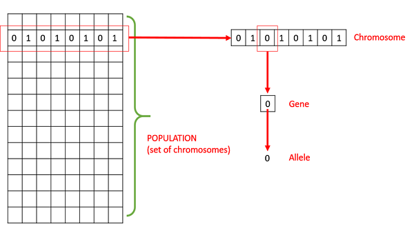
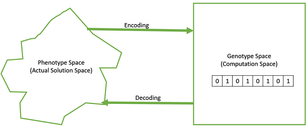
Genotype − Genotype is the population in the computation space. In the computation space, the solutions are represented in a way which can be easily understood and manipulated using a computing system.
Phenotype − Phenotype is the population in the actual real world solution space in which solutions are represented in a way they are represented in real world situations.
Decoding and Encoding − For simple problems, the phenotype and genotype spaces are the same. However, in most of the cases, the phenotype and genotype spaces are different. Decoding is a process of transforming a solution from the genotype to the phenotype space, while encoding is a process of transforming from the phenotype to genotype space. Decoding should be fast as it is carried out repeatedly in a GA during the fitness value calculation.
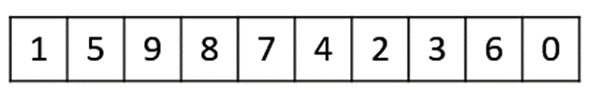
For example, consider the 0/1 Knapsack Problem. The Phenotype space consists of solutions which just contain the item numbers of the items to be picked.
However, in the genotype space it can be represented as a binary string of length n (where n is the number of items). A 0 at position x represents that xth item is picked while a 1 represents the reverse. This is a case where genotype and phenotype spaces are different.
Fitness Function − A fitness function simply defined is a function which takes the solution as input and produces the suitability of the solution as the output. In some cases, the fitness function and the objective function may be the same, while in others it might be different based on the problem.
Genetic Operators − These alter the genetic composition of the offspring. These include crossover, mutation, selection, etc.
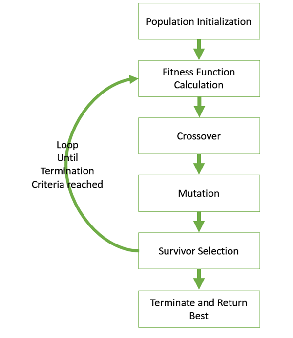
Basic Structure
The basic structure of a GA is as follows −
We start with an initial population (which may be generated at random or seeded by other heuristics), select parents from this population for mating. Apply crossover and mutation operators on the parents to generate new off-springs. And finally these off-springs replace the existing individuals in the population and the process repeats. In this way genetic algorithms actually try to mimic the human evolution to some extent.
Each of the following steps are covered as a separate chapter later in this tutorial.
A generalized pseudo-code for a GA is explained in the following program −
GA()
   initialize population
   find fitness of population

   while (termination criteria is reached) do
      parent selection
      crossover with probability pc
      mutation with probability pm
      decode and fitness calculation
      survivor selection
      find best
   return best
Genotype Representation
One of the most important decisions to make while implementing a genetic algorithm is deciding the representation that we will use to represent our solutions. It has been observed that improper representation can lead to poor performance of the GA.
Therefore, choosing a proper representation, having a proper definition of the mappings between the phenotype and genotype spaces is essential for the success of a GA.
In this section, we present some of the most commonly used representations for genetic algorithms. However, representation is highly problem specific and the reader might find that another representation or a mix of the representations mentioned here might suit his/her problem better.
Binary Representation
This is one of the simplest and most widely used representation in GAs. In this type of representation the genotype consists of bit strings.
For some problems when the solution space consists of Boolean decision variables yes or no, the binary representation is natural. Take for example the 0/1 Knapsack Problem. If there are n items, we can represent a solution by a binary string of n elements, where the xth element tells whether the item x is picked (1) or not (0).
For other problems, specifically those dealing with numbers, we can represent the numbers with their binary representation. The problem with this kind of encoding is that different bits have different significance and therefore mutation and crossover operators can have undesired consequences. This can be resolved to some extent by using Gray Coding, as a change in one bit does not have a massive effect on the solution.
Real Valued Representation
For problems where we want to define the genes using continuous rather than discrete variables, the real valued representation is the most natural. The precision of these real valued or floating point numbers is however limited to the computer.
Integer Representation
For discrete valued genes, we cannot always limit the solution space to binary yes or no. For example, if we want to encode the four distances North, South, East and West, we can encode them as {0,1,2,3}. In such cases, integer representation is desirable.
Permutation Representation
In many problems, the solution is represented by an order of elements. In such cases permutation representation is the most suited.
A classic example of this representation is the travelling salesman problem (TSP). In this the salesman has to take a tour of all the cities, visiting each city exactly once and come back to the starting city. The total distance of the tour has to be minimized. The solution to this TSP is naturally an ordering or permutation of all the cities and therefore using a permutation representation makes sense for this problem.
Genetic Algorithms - Population
Population is a subset of solutions in the current generation. It can also be defined as a set of chromosomes. There are several things to be kept in mind when dealing with GA population −
The diversity of the population should be maintained otherwise it might lead to premature convergence.
The population size should not be kept very large as it can cause a GA to slow down, while a smaller population might not be enough for a good mating pool. Therefore, an optimal population size needs to be decided by trial and error.
The population is usually defined as a two dimensional array of size population, size x, chromosome size.
Population Initialization
There are two primary methods to initialize a population in a GA. They are −
Random Initialization − Populate the initial population with completely random solutions.
Heuristic initialization − Populate the initial population using a known heuristic for the problem.
It has been observed that the entire population should not be initialized using a heuristic, as it can result in the population having similar solutions and very little diversity. It has been experimentally observed that the random solutions are the ones to drive the population to optimality. Therefore, with heuristic initialization, we just seed the population with a couple of good solutions, filling up the rest with random solutions rather than filling the entire population with heuristic based solutions.
It has also been observed that heuristic initialization in some cases, only effects the initial fitness of the population, but in the end, it is the diversity of the solutions which lead to optimality.
Population Models
There are two population models widely in use −
Steady State
In steady state GA, we generate one or two off-springs in each iteration and they replace one or two individuals from the population. A steady state GA is also known as Incremental GA.
Generational
In a generational model, we generate n off-springs, where n is the population size, and the entire population is replaced by the new one at the end of the iteration.
Genetic Algorithms - Fitness Function
The fitness function simply defined is a function which takes a candidate solution to the problem as input and produces as output how fit our how good the solution is with respect to the problem in consideration.
Calculation of fitness value is done repeatedly in a GA and therefore it should be sufficiently fast. A slow computation of the fitness value can adversely affect a GA and make it exceptionally slow.
In most cases the fitness function and the objective function are the same as the objective is to either maximize or minimize the given objective function. However, for more complex problems with multiple objectives and constraints, an Algorithm Designer might choose to have a different fitness function.
A fitness function should possess the following characteristics −
The fitness function should be sufficiently fast to compute.
It must quantitatively measure how fit a given solution is or how fit individuals can be produced from the given solution.
In some cases, calculating the fitness function directly might not be possible due to the inherent complexities of the problem at hand. In such cases, we do fitness approximation to suit our needs.
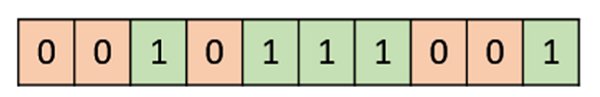
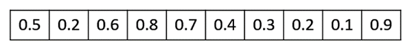
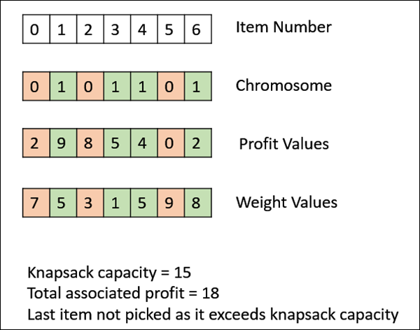
The following image shows the fitness calculation for a solution of the 0/1 Knapsack. It is a simple fitness function which just sums the profit values of the items being picked (which have a 1), scanning the elements from left to right till the knapsack is full.
Genetic Algorithms - Parent Selection
Parent Selection is the process of selecting parents which mate and recombine to create off-springs for the next generation. Parent selection is very crucial to the convergence rate of the GA as good parents drive individuals to a better and fitter solutions.
However, care should be taken to prevent one extremely fit solution from taking over the entire population in a few generations, as this leads to the solutions being close to one another in the solution space thereby leading to a loss of diversity. Maintaining good diversity in the population is extremely crucial for the success of a GA. This taking up of the entire population by one extremely fit solution is known as premature convergence and is an undesirable condition in a GA.
Fitness Proportionate Selection
Fitness Proportionate Selection is one of the most popular ways of parent selection. In this every individual can become a parent with a probability which is proportional to its fitness. Therefore, fitter individuals have a higher chance of mating and propagating their features to the next generation. Therefore, such a selection strategy applies a selection pressure to the more fit individuals in the population, evolving better individuals over time.
Consider a circular wheel. The wheel is divided into n pies, where n is the number of individuals in the population. Each individual gets a portion of the circle which is proportional to its fitness value.
Two implementations of fitness proportionate selection are possible −
Roulette Wheel Selection
In a roulette wheel selection, the circular wheel is divided as described before. A fixed point is chosen on the wheel circumference as shown and the wheel is rotated. The region of the wheel which comes in front of the fixed point is chosen as the parent. For the second parent, the same process is repeated.
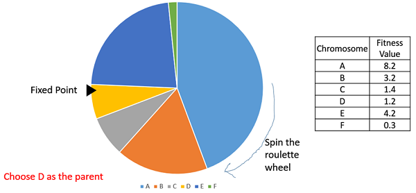
It is clear that a fitter individual has a greater pie on the wheel and therefore a greater chance of landing in front of the fixed point when the wheel is rotated. Therefore, the probability of choosing an individual depends directly on its fitness.
Implementation wise, we use the following steps −
Calculate S = the sum of a finesses.
Generate a random number between 0 and S.
Starting from the top of the population, keep adding the finesses to the partial sum P, till P<S.
The individual for which P exceeds S is the chosen individual.
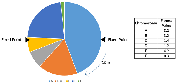
Stochastic Universal Sampling (SUS)
Stochastic Universal Sampling is quite similar to Roulette wheel selection, however instead of having just one fixed point, we have multiple fixed points as shown in the following image. Therefore, all the parents are chosen in just one spin of the wheel. Also, such a setup encourages the highly fit individuals to be chosen at least once.
It is to be noted that fitness proportionate selection methods dont work for cases where the fitness can take a negative value.
Tournament Selection
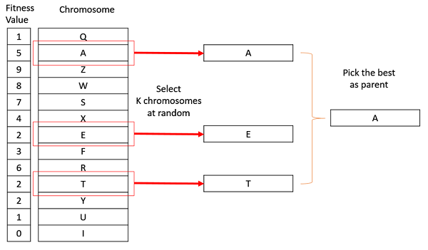
In K-Way tournament selection, we select K individuals from the population at random and select the best out of these to become a parent. The same process is repeated for selecting the next parent. Tournament Selection is also extremely popular in literature as it can even work with negative fitness values.
Rank Selection
Rank Selection also works with negative fitness values and is mostly used when the individuals in the population have very close fitness values (this happens usually at the end of the run). This leads to each individual having an almost equal share of the pie (like in case of fitness proportionate selection) as shown in the following image and hence each individual no matter how fit relative to each other has an approximately same probability of getting selected as a parent. This in turn leads to a loss in the selection pressure towards fitter individuals, making the GA to make poor parent selections in such situations.
In this, we remove the concept of a fitness value while selecting a parent. However, every individual in the population is ranked according to their fitness. The selection of the parents depends on the rank of each individual and not the fitness. The higher ranked individuals are preferred more than the lower ranked ones.
| Chromosome | Fitness Value | Rank |
|---|---|---|
| A | 8.1 | 1 |
| B | 8.0 | 4 |
| C | 8.05 | 2 |
| D | 7.95 | 6 |
| E | 8.02 | 3 |
| F | 7.99 | 5 |
Random Selection
In this strategy we randomly select parents from the existing population. There is no selection pressure towards fitter individuals and therefore this strategy is usually avoided.
Genetic Algorithms - Crossover
In this chapter, we will discuss about what a Crossover Operator is along with its other modules, their uses and benefits.
Introduction to Crossover
The crossover operator is analogous to reproduction and biological crossover. In this more than one parent is selected and one or more off-springs are produced using the genetic material of the parents. Crossover is usually applied in a GA with a high probability pc .
Crossover Operators
In this section we will discuss some of the most popularly used crossover operators. It is to be noted that these crossover operators are very generic and the GA Designer might choose to implement a problem-specific crossover operator as well.
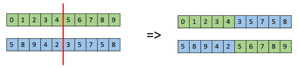
One Point Crossover
In this one-point crossover, a random crossover point is selected and the tails of its two parents are swapped to get new off-springs.
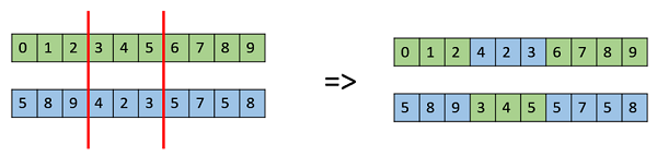
Multi Point Crossover
Multi point crossover is a generalization of the one-point crossover wherein alternating segments are swapped to get new off-springs.
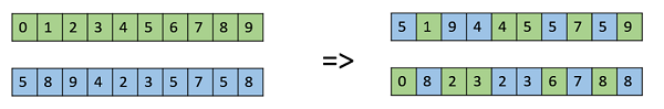
Uniform Crossover
In a uniform crossover, we dont divide the chromosome into segments, rather we treat each gene separately. In this, we essentially flip a coin for each chromosome to decide whether or not itll be included in the off-spring. We can also bias the coin to one parent, to have more genetic material in the child from that parent.
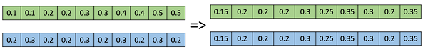
Whole Arithmetic Recombination
This is commonly used for integer representations and works by taking the weighted average of the two parents by using the following formulae −
- Child1 = α.x + (1-α).y
- Child2 = α.x + (1-α).y
Obviously, if α = 0.5, then both the children will be identical as shown in the following image.
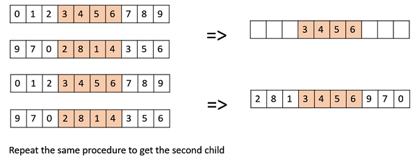
Davis Order Crossover (OX1)
OX1 is used for permutation based crossovers with the intention of transmitting information about relative ordering to the off-springs. It works as follows −
Create two random crossover points in the parent and copy the segment between them from the first parent to the first offspring.
Now, starting from the second crossover point in the second parent, copy the remaining unused numbers from the second parent to the first child, wrapping around the list.
Repeat for the second child with the parents role reversed.
There exist a lot of other crossovers like Partially Mapped Crossover (PMX), Order based crossover (OX2), Shuffle Crossover, Ring Crossover, etc.
Genetic Algorithms - Mutation
Introduction to Mutation
In simple terms, mutation may be defined as a small random tweak in the chromosome, to get a new solution. It is used to maintain and introduce diversity in the genetic population and is usually applied with a low probability pm. If the probability is very high, the GA gets reduced to a random search.
Mutation is the part of the GA which is related to the exploration of the search space. It has been observed that mutation is essential to the convergence of the GA while crossover is not.
Mutation Operators
In this section, we describe some of the most commonly used mutation operators. Like the crossover operators, this is not an exhaustive list and the GA designer might find a combination of these approaches or a problem-specific mutation operator more useful.
Bit Flip Mutation
In this bit flip mutation, we select one or more random bits and flip them. This is used for binary encoded GAs.

Random Resetting
Random Resetting is an extension of the bit flip for the integer representation. In this, a random value from the set of permissible values is assigned to a randomly chosen gene.
Swap Mutation
In swap mutation, we select two positions on the chromosome at random, and interchange the values. This is common in permutation based encodings.

Scramble Mutation
Scramble mutation is also popular with permutation representations. In this, from the entire chromosome, a subset of genes is chosen and their values are scrambled or shuffled randomly.

Inversion Mutation
In inversion mutation, we select a subset of genes like in scramble mutation, but instead of shuffling the subset, we merely invert the entire string in the subset.

Genetic Algorithms - Survivor Selection
The Survivor Selection Policy determines which individuals are to be kicked out and which are to be kept in the next generation. It is crucial as it should ensure that the fitter individuals are not kicked out of the population, while at the same time diversity should be maintained in the population.
Some GAs employ Elitism. In simple terms, it means the current fittest member of the population is always propagated to the next generation. Therefore, under no circumstance can the fittest member of the current population be replaced.
The easiest policy is to kick random members out of the population, but such an approach frequently has convergence issues, therefore the following strategies are widely used.
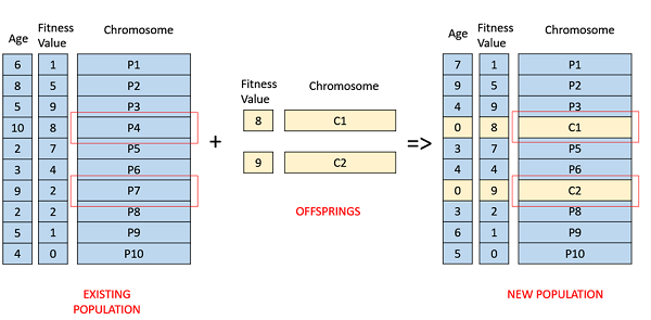
Age Based Selection
In Age-Based Selection, we dont have a notion of a fitness. It is based on the premise that each individual is allowed in the population for a finite generation where it is allowed to reproduce, after that, it is kicked out of the population no matter how good its fitness is.
For instance, in the following example, the age is the number of generations for which the individual has been in the population. The oldest members of the population i.e. P4 and P7 are kicked out of the population and the ages of the rest of the members are incremented by one.
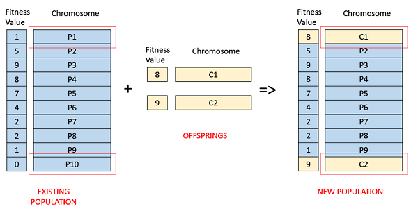
Fitness Based Selection
In this fitness based selection, the children tend to replace the least fit individuals in the population. The selection of the least fit individuals may be done using a variation of any of the selection policies described before tournament selection, fitness proportionate selection, etc.
For example, in the following image, the children replace the least fit individuals P1 and P10 of the population. It is to be noted that since P1 and P9 have the same fitness value, the decision to remove which individual from the population is arbitrary.
Genetic Algorithms - Termination Condition
The termination condition of a Genetic Algorithm is important in determining when a GA run will end. It has been observed that initially, the GA progresses very fast with better solutions coming in every few iterations, but this tends to saturate in the later stages where the improvements are very small. We usually want a termination condition such that our solution is close to the optimal, at the end of the run.
Usually, we keep one of the following termination conditions −
- When there has been no improvement in the population for X iterations.
- When we reach an absolute number of generations.
- When the objective function value has reached a certain pre-defined value.
For example, in a genetic algorithm we keep a counter which keeps track of the generations for which there has been no improvement in the population. Initially, we set this counter to zero. Each time we dont generate off-springs which are better than the individuals in the population, we increment the counter.
However, if the fitness any of the off-springs is better, then we reset the counter to zero. The algorithm terminates when the counter reaches a predetermined value.
Like other parameters of a GA, the termination condition is also highly problem specific and the GA designer should try out various options to see what suits his particular problem the best.
Models Of Lifetime Adaptation
Till now in this tutorial, whatever we have discussed corresponds to the Darwinian model of evolution natural selection and genetic variation through recombination and mutation. In nature, only the information contained in the individuals genotype can be transmitted to the next generation. This is the approach which we have been following in the tutorial so far.
However, other models of lifetime adaptation Lamarckian Model and Baldwinian Model also do exist. It is to be noted that whichever model is the best, is open for debate and the results obtained by researchers show that the choice of lifetime adaptation is highly problem specific.
Often, we hybridize a GA with local search like in Memetic Algorithms. In such cases, one might choose do go with either Lamarckian or Baldwinian Model to decide what to do with individuals generated after the local search.
Lamarckian Model
The Lamarckian Model essentially says that the traits which an individual acquires in his/her lifetime can be passed on to its offspring. It is named after French biologist Jean-Baptiste Lamarck.
Even though, natural biology has completely disregarded Lamarckism as we all know that only the information in the genotype can be transmitted. However, from a computation view point, it has been shown that adopting the Lamarckian model gives good results for some of the problems.
In the Lamarckian model, a local search operator examines the neighborhood (acquiring new traits), and if a better chromosome is found, it becomes the offspring.
Baldwinian Model
The Baldwinian model is an intermediate idea named after James Mark Baldwin (1896). In the Baldwin model, the chromosomes can encode a tendency of learning beneficial behaviors. This means, that unlike the Lamarckian model, we dont transmit the acquired traits to the next generation, and neither do we completely ignore the acquired traits like in the Darwinian Model.
The Baldwin Model is in the middle of these two extremes, wherein the tendency of an individual to acquire certain traits is encoded rather than the traits themselves.
In this Baldwinian Model, a local search operator examines the neighborhood (acquiring new traits), and if a better chromosome is found, it only assigns the improved fitness to the chromosome and does not modify the chromosome itself. The change in fitness signifies the chromosomes capability to acquire the trait, even though it is not passed directly to the future generations.
Effective Implementation
GAs are very general in nature, and just applying them to any optimization problem wouldnt give good results. In this section, we describe a few points which would help and assist a GA designer or GA implementer in their work.
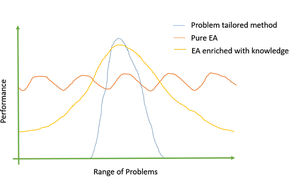
Introduce problem-specific domain knowledge
It has been observed that the more problem-specific domain knowledge we incorporate into the GA; the better objective values we get. Adding problem specific information can be done by either using problem specific crossover or mutation operators, custom representations, etc.
The following image shows Michalewiczs (1990) view of the EA −
Reduce Crowding
Crowding happens when a highly fit chromosome gets to reproduce a lot, and in a few generations, the entire population is filled with similar solutions having similar fitness. This reduces diversity which is a very crucial element to ensure the success of a GA. There are numerous ways to limit crowding. Some of them are −
Mutation to introduce diversity.
Switching to rank selection and tournament selection which have more selection pressure than fitness proportionate selection for individuals with similar fitness.
Fitness Sharing − In this an individuals fitness is reduced if the population already contains similar individuals.
Randomization Helps!
It has been experimentally observed that the best solutions are driven by randomized chromosomes as they impart diversity to the population. The GA implementer should be careful to keep sufficient amount of randomization and diversity in the population for the best results.
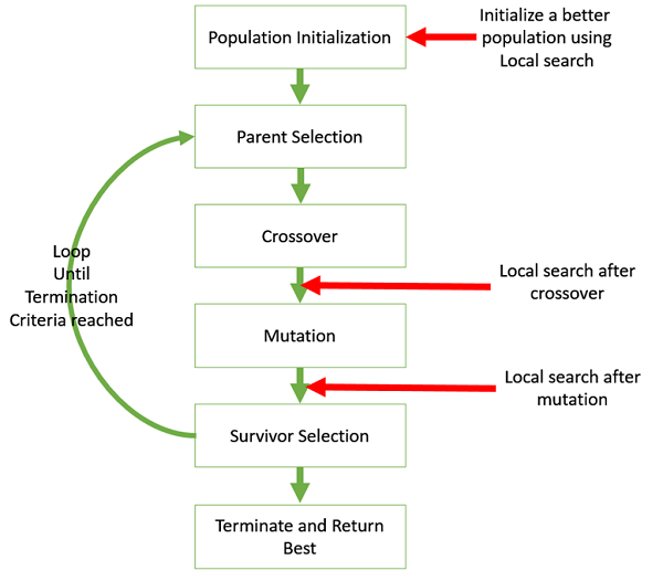
Hybridize GA with Local Search
Local search refers to checking the solutions in the neighborhood of a given solution to look for better objective values.
It may be sometimes useful to hybridize the GA with local search. The following image shows the various places in which local search can be introduced in a GA.
Variation of parameters and techniques
In genetic algorithms, there is no one size fits all or a magic formula which works for all problems. Even after the initial GA is ready, it takes a lot of time and effort to play around with the parameters like population size, mutation and crossover probability etc. to find the ones which suit the particular problem.
Genetic Algorithms - Advanced Topics
In this section, we introduce some advanced topics in Genetic Algorithms. A reader looking for just an introduction to GAs may choose to skip this section.
Constrained Optimization Problems
Constrained Optimization Problems are those optimization problems in which we have to maximize or minimize a given objective function value that is subject to certain constraints. Therefore, not all results in the solution space are feasible, and the solution space contains feasible regions as shown in the following image.
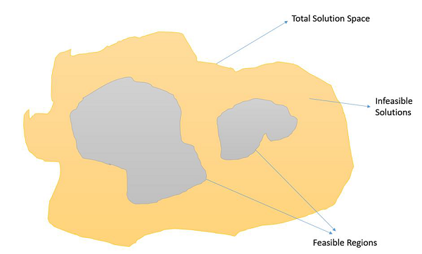
In such a scenario, crossover and mutation operators might give us solutions which are infeasible. Therefore, additional mechanisms have to be employed in the GA when dealing with constrained Optimization Problems.
Some of the most common methods are −
Using penalty functions which reduces the fitness of infeasible solutions, preferably so that the fitness is reduced in proportion with the number of constraints violated or the distance from the feasible region.
Using repair functions which take an infeasible solution and modify it so that the violated constraints get satisfied.
Not allowing infeasible solutions to enter into the population at all.
Use a special representation or decoder functions that ensures feasibility of the solutions.
Basic Theoretical Background
In this section, we will discuss about the Schema and NFL theorem along with the building block hypothesis.
Schema Theorem
Researchers have been trying to figure out the mathematics behind the working of genetic algorithms, and Hollands Schema Theorem is a step in that direction. Over the years various improvements and suggestions have been done to the Schema Theorem to make it more general.
In this section, we dont delve into the mathematics of the Schema Theorem, rather we try to develop a basic understanding of what the Schema Theorem is. The basic terminology to know are as follows −
A Schema is a template. Formally, it is a string over the alphabet = {0,1,*},
where * is dont care and can take any value.
Therefore, *10*1 could mean 01001, 01011, 11001, or 11011
Geometrically, a schema is a hyper-plane in the solution search space.
Order of a schema is the number of specified fixed positions in a gene.
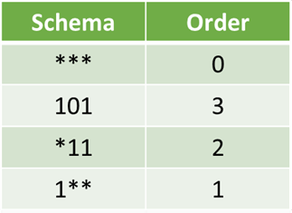
Defining length is the distance between the two furthest fixed symbols in the gene.
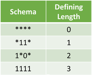
The schema theorem states that this schema with above average fitness, short defining length and lower order is more likely to survive crossover and mutation.
Building Block Hypothesis
Building Blocks are low order, low defining length schemata with the above given average fitness. The building block hypothesis says that such building blocks serve as a foundation for the GAs success and adaptation in GAs as it progresses by successively identifying and recombining such building blocks.
No Free Lunch (NFL) Theorem
Wolpert and Macready in 1997 published a paper titled "No Free Lunch Theorems for Optimization." It essentially states that if we average over the space of all possible problems, then all non-revisiting black box algorithms will exhibit the same performance.
It means that the more we understand a problem, our GA becomes more problem specific and gives better performance, but it makes up for that by performing poorly for other problems.
GA Based Machine Learning
Genetic Algorithms also find application in Machine Learning. Classifier systems are a form of genetics-based machine learning (GBML) system that are frequently used in the field of machine learning. GBML methods are a niche approach to machine learning.
There are two categories of GBML systems −
The Pittsburg Approach − In this approach, one chromosome encoded one solution, and so fitness is assigned to solutions.
The Michigan Approach − one solution is typically represented by many chromosomes and so fitness is assigned to partial solutions.
It should be kept in mind that the standard issue like crossover, mutation, Lamarckian or Darwinian, etc. are also present in the GBML systems.
Genetic Algorithms - Application Areas
Genetic Algorithms are primarily used in optimization problems of various kinds, but they are frequently used in other application areas as well.
In this section, we list some of the areas in which Genetic Algorithms are frequently used. These are −
Optimization − Genetic Algorithms are most commonly used in optimization problems wherein we have to maximize or minimize a given objective function value under a given set of constraints. The approach to solve Optimization problems has been highlighted throughout the tutorial.
Economics − GAs are also used to characterize various economic models like the cobweb model, game theory equilibrium resolution, asset pricing, etc.
Neural Networks − GAs are also used to train neural networks, particularly recurrent neural networks.
Parallelization − GAs also have very good parallel capabilities, and prove to be very effective means in solving certain problems, and also provide a good area for research.
Image Processing − GAs are used for various digital image processing (DIP) tasks as well like dense pixel matching.
Vehicle routing problems − With multiple soft time windows, multiple depots and a heterogeneous fleet.
Scheduling applications − GAs are used to solve various scheduling problems as well, particularly the time tabling problem.
Machine Learning − as already discussed, genetics based machine learning (GBML) is a niche area in machine learning.
Robot Trajectory Generation − GAs have been used to plan the path which a robot arm takes by moving from one point to another.
Parametric Design of Aircraft − GAs have been used to design aircrafts by varying the parameters and evolving better solutions.
DNA Analysis − GAs have been used to determine the structure of DNA using spectrometric data about the sample.
Multimodal Optimization − GAs are obviously very good approaches for multimodal optimization in which we have to find multiple optimum solutions.
Traveling salesman problem and its applications − GAs have been used to solve the TSP, which is a well-known combinatorial problem using novel crossover and packing strategies.
Genetic Algorithms - Further Readings
The following books can be referred to further enhance the readers knowledge of Genetic Algorithms, and Evolutionary Computation in general −
Genetic Algorithms in Search, Optimization and Machine Learning by David E. Goldberg.
Genetic Algorithms + Data Structures = Evolutionary Programs by Zbigniew Michalewicz.
Practical Genetic Algorithms by Randy L. Haupt and Sue Ellen Haupt.
Multi Objective Optimization using Evolutionary Algorithms by Kalyanmoy Deb.
