- Excel Power Pivot - Home
- Excel Power Pivot - Overview
- Excel Power Pivot - Installing
- Excel Power Pivot - Features
- Excel Power Pivot - Loading Data
- Excel Power Pivot - Data Model
- Power Pivot - Managing Data Model
- Excel Power Pivot Table - Creation
- Excel Power Pivot - Basics of DAX
- Power Pivot Table - Exploring Data
- Excel Power Pivot Table - Flattened
- Excel Power Pivot Charts - Creation
- Table & Chart Combinations
- Excel Power Pivot - Hierarchies
- Power Pivot - Aesthetic Reports
- Excel Power Pivot Useful Resources
- Excel Power Pivot - Quick Guide
- Excel Power Pivot - Resources
- Excel Power Pivot - Discussion
Excel Power Pivot - Flattened
When the data has many levels, sometimes it becomes cumbersome to read the PivotTable report.
For example, consider the following Data Model.
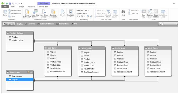
We will create a Power PivotTable and a Power Flattened PivotTable to get an understanding of the layouts.
Creating a PivotTable
You can create a Power PivotTable as follows −
Click the Home tab on the Ribbon in the PowerPivot window.
Click PivotTable.
Select PivotTable from the dropdown list.
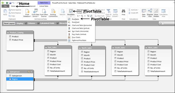
An empty PivotTable will be created.
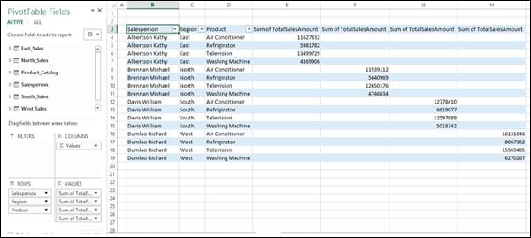
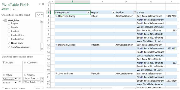
Drag the fields − Salesperson, Region and Product from the PivotTable Fields list to the ROWS area.
Drag the field − TotalSalesAmount from the Tables − East, North, South and West to the ∑ VALUES area.
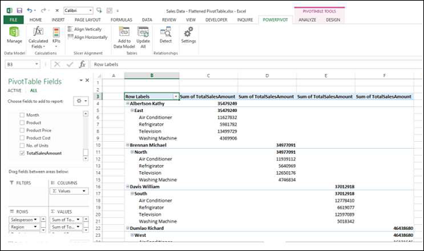
As you can see, it is a bit cumbersome read such a report. If the number of entries becomes more, the more difficult it will be.
Power Pivot provides a solution for a better representation of data with Flattened PivotTable.
Creating a Flattened PivotTable
You can create a Power Flattened PivotTable as follows −
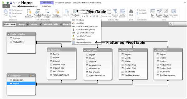
Click the Home tab on the Ribbon in the PowerPivot window.
Click PivotTable.
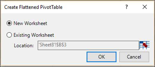
Select Flattened PivotTable from the dropdown list.
Create Flattened PivotTable dialog box appears. Select New Worksheet and click OK.
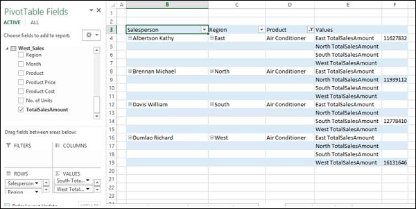
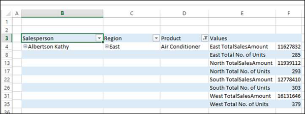
As you can observe the data is flattened out in this PivotTable.
Note − In this case Salesperson, Region and Product are in ROWS area only as in the previous case. However, in the PivotTable layout, these three fields are appearing as three columns.
Exploring Data in Flattened PivotTable
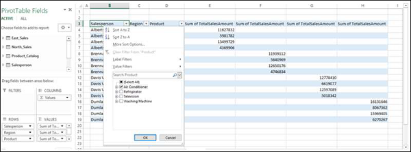
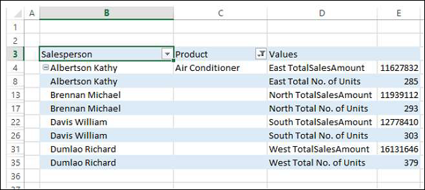
Suppose you want to summarize the sales data for the product − Air Conditioner. You can do it in a simple way with the Flattened PivotTable as follows −
Click the arrow next to the column header − Product.
Check the box Air Conditioner and uncheck the other boxes. Click OK.
The Flattened PivotTable is filtered to the Air Conditioner sales data.
You can make it look more flattened by dragging ∑ VALUES to ROWS area from the COLUMNS area.
Rename the custom names of the summation values in the ∑ VALUES area to make them more meaningful as follows −
Click on a summation value, say, Sum of TotalSalesAmount for East.
Select Value Field Settings from the dropdown list.
Change the Custom Name to East TotalSalesAmount.
Repeat the steps for the other three summation values.
You can also summarize the number of units sold.
Drag No. of Units to the ∑ VALUES area from each of the tables − East_Sales, North_Sales, South_Sales and West_Sales.
Rename the values to East Total No. of Units, North Total No. of Units, South Total No. of Units and West Total No. of Units respectively.
As you can observe, in both of the above tables, there are rows with empty values, as each salesperson represents a single region and each region is represented only by a single salesperson.
Select the rows with empty values.
Right click and click on Hide in the dropdown list.
All the rows with empty values will be hidden.
As you can observe, though the rows with empty values are not displayed, the information on the Salesperson also got hidden.
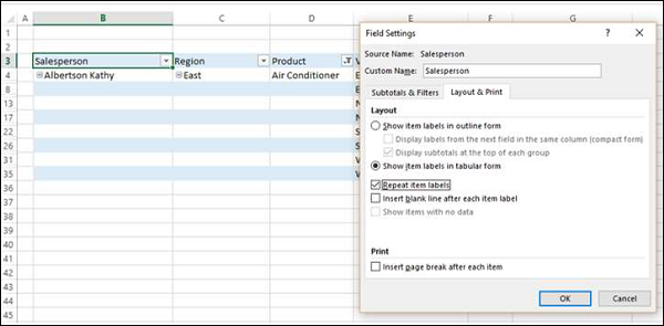
Click on the column header − Salesperson.
Click the ANALYZE tab on the Ribbon.
Click Field Settings. The Field Settings dialog box appears.
Click the Layout & Print tab.
Check the box - Repeat Item Labels.
Click OK.
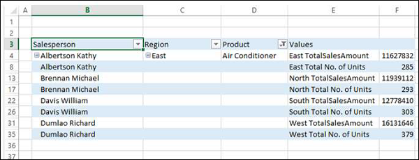
As you can observe, the Salesperson information is displayed and the rows with empty values are hidden. Further, the column Region in the report is redundant, as the values in the Values column are self-explanatory.
Drag the field Regions out of Area.
Reverse the order of the fields − Salesperson and Product in the ROWS area.
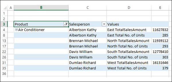
You have arrived at a concise report combining data from six tables in the Power Pivot.
