Excel DAX - Ranking and Comparing Values

---

If you want to show only the top n number of items in a column or PivotTable, you have the following two options −

• You can select n number of top values in the PivotTable.

• You can create a DAX formula that dynamically ranks values and then uses the ranking values in a Slicer.

Applying a Filter to Show only the Top Few Items

To select n number of top values for display in the PivotTable, do the following −

• Click the down arrow in the row labels heading in the PivotTable.
• Click the Value Filters in the dropdown list and then click Top 10.

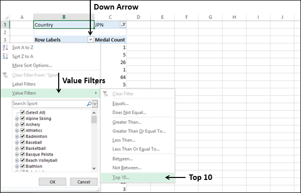
Top 10 Filter (<column name>) dialog box appears.

• Under Show, select the following in the boxes from left to right.
  • Top
  • 18 (The number of top values that you want to display. The default is 10.)
  • Items.
  • In the by box, select Medal Count.

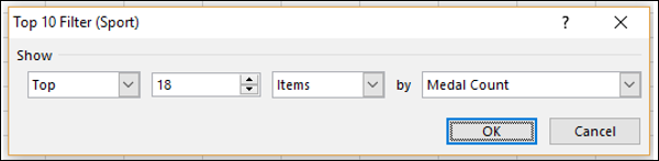
• Click OK. The top 18 values will be displayed in the PivotTable.

Advantages and Disadvantages of Applying Filter

Advantages

• It is simple and easy to use.
• Suitable for tables with large number of rows.

Disadvantages

• The filter is solely for display purposes.

• If the data underlying the PivotTable changes, you must manually refresh the PivotTable to see the changes.

Creating a DAX Formula That Dynamically Ranks Values

You can create a calculated column using a DAX formula that contains the ranked values. You can then use a slicer on the resulting calculated column to select the values to be displayed.

You can obtain a rank value for a given value in a row by counting the number of rows in the same table having a value larger than the one that is being compared. This method returns the following −

• A zero value for the highest value in the table.

• Equal values will have the same rank value. If n number of values are equal, the next value after the equal values will have a nonconsecutive rank value adding up the number n.

For example, if you have a table ‘Sales’ with sales data, you can create a calculated column with the ranks of the Sales Amount values as follows −

= COUNTROWS (FILTER (Sales,  
   EARLIER (Sales [Sales Amount]) < Sales [Sales Amount])
) + 1 

Next, you can insert a Slicer on the new calculated column and selectively display the values by ranks.

Advantages and Disadvantages of Dynamic Ranks

Advantages

• The ranking is done in the table and not on a PivotTable. Hence, can be used in any number of PivotTables.

• DAX formulas are calculated dynamically. Hence, you can always be sure that the ranking is correct even if the underlying data has changed.

• Since the DAX formula is used in a calculated column, you can use the ranking in a Slicer.

• Suitable for tables with large number of rows.

Disadvantages

Since the DAX calculations are computationally expensive, this method might not be suitable for tables with large number of rows.