Electric Traction: Trapezoidal Speed Time Curve

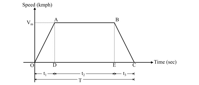
The speed-time curve of a main line service is best and most easily replaced by trapezoid. The figure shows the simplified trapezoidal speed-time curve for the main line service.

Let,

• $\mathit{V_{m}}$ = Crest speed in kmph

• $\alpha$ = Acceleration in kmphps

• $\beta$ = Retardation in kmphps

• T = Total time of run in seconds

• $\mathit{t_{\mathrm{1}}}$ = Acceleration time in seconds

• $\mathit{t_{\mathrm{2}}}$ = Free running time in seconds

• $\mathit{t_{\mathrm{3}}}$ = Retardation time in seconds

• D = Total distance of run in km

Therefore, the time of acceleration in seconds is given by,

$$\mathrm{\mathit{t_{\mathrm{1}}}\:=\:\frac{\mathit{V_{m}}}{\alpha }}$$

And the time for retardation in seconds is,

$$\mathrm{\mathit{t_{\mathrm{3}}}\:=\:\frac{\mathit{V_{m}}}{\beta }}$$

Hence, the time for free running in seconds is,

$$\mathrm{\mathit{t_{\mathrm{2}}}\:=\:\mathit{T}-\mathrm{\left (\mathit{t_{\mathrm{1}}} +\mathit{t_{\mathrm{2}}} \right )}\:=\:\mathit{T}-\mathrm{\left ( \frac{\mathit{V_{m}}}{\alpha }+\frac{\mathit{V_{m}}}{\beta } \right )}}$$

Now, the total distance of run in km is,

$$\mathrm{\mathit{D}\:=\:\mathrm{distance\: travelled \:during \:acceleration\:+\:distance \:travelled \:during\: free\: run\:+\:distnace \:travelled\: during\: braking\: retardation}}$$

$$\mathrm{\Rightarrow \mathit{D}\:=\:\mathrm{Area\: of\: OABC\:=\:Area \:of\:\triangle AOD\:+\:Area\: of\: rectangle\: DABE\:+\:Area of \triangle CBE}}$$

$$\mathrm{\Rightarrow \mathit{D}\:=\:\mathrm{\left ( \frac{1}{2}\times \mathit{V_{m}}\times \frac{\mathit{t_{\mathrm{1}}}}{3600} \right )}\:+\:\mathrm{\left ( \mathit{V_{m}}\times\frac{\mathit{t_{\mathrm{2}}}}{3600} \right )}\:+\:\mathrm{\left ( \frac{1}{2}\times \mathit{V_{m}}\times \frac{\mathit{t_{\mathrm{3}}}}{3600} \right )}}$$

On substituting the values of t₁, t₂ and t₃, we get,

$$\mathrm{\mathit{D}\:=\:\frac{\mathit{V_{m}^{\mathrm{2}}}}{7200\alpha}\:+\:\frac{\mathit{V_{m}} }{3600}\mathrm{\left [\mathit{T}-\mathrm{\left ( \frac{\mathit{V_{m}}}{\alpha }+\frac{\mathit{V_{m}}}{\beta } \right )} \right ]}\:+\:\frac{\mathit{V_{m}^{\mathrm{2}}}}{7200\beta }}$$

$$\mathrm{\Rightarrow \mathit{D}\:=\:\frac{\mathit{V_{m}^{\mathrm{2}}}}{7200\alpha}\:+\:\frac{\mathit{V_{m}} }{3600}\mathit{T}-\frac{\mathit{V_{m}^{\mathrm{2}}}}{3600\alpha}-\frac{\mathit{V_{m}^{\mathrm{2}}}}{3600\beta}+\frac{\mathit{V_{m}^{\mathrm{2}}}}{7200\beta}}$$

$$\mathrm{\Rightarrow \mathit{D}\:=\:\frac{\mathit{V_{m}} }{3600}\mathit{T}-\frac{\mathit{V_{m}^{\mathrm{2}}}}{7200\alpha}-\frac{\mathit{V_{m}^{\mathrm{2}}}}{7200\beta}}$$

$$\mathrm{\Rightarrow \frac{\mathit{V_{m}^{\mathrm{2}}}}{3600}\mathrm{\left ( \frac{1}{2\alpha } +\frac{1}{2\beta }\right )}-\frac{\mathit{V_{m}}}{3600}\mathit{T}\:+\:\mathit{D}\:=\:0}$$

$$\mathrm{\Rightarrow \mathit{V_{m}^{\mathrm{2}}}\mathrm{\left ( \frac{1}{2\alpha } +\frac{1}{2\beta } \right )}-\mathit{V_{m}}\mathit{T}\:+\:3600\mathit{D}\:=\:0\:\:\:\cdot \cdot \cdot \mathrm{\left ( 1 \right )}}$$

Equation (1) is the quadratic equation for $\mathit{V_{m}}$

On substituting $\mathrm{\left ( \frac{1}{2\alpha } +\frac{1}{2\beta } \right )}\:=\:\mathit{K}$ we get,

$$\mathrm{\mathit{KV_{m}^{\mathrm{2}}}-\mathit{V_{m}\mathit{T}}\:+\:3600\mathit{D}\:=\:0}$$

$$\mathrm{\Rightarrow \mathit{V_{m}\:=\:\frac{\mathit{T}\pm \sqrt{T^{\mathrm{2}}-\mathrm{4}\mathit{K}\times \mathrm{3600}\mathrm{D}}}{\mathrm{2}\mathit{K}}}}$$

$$\mathrm{\Rightarrow \mathit{V_{m}\:=\:\frac{\mathit{T}}{\mathrm{2}\mathit{K}}\pm \sqrt{\frac{\mathit{T^{2}}}{\mathrm{4}K^{\mathrm{2}}}-\frac{\mathrm{3600D}}{\mathit{K}}}}}$$

Here, the +ve sign cannot be adopted because the value of Vm obtained by using +ve sign will be much higher than that is possible in practice. Therefore, negative sign is used and we get,

$$\mathrm{\mathit{V_{m}\:=\:\frac{\mathit{T}}{\mathrm{2}\mathit{K}}- \sqrt{\frac{\mathit{T^{\mathrm{2}}}}{\mathrm{4}K^{\mathrm{2}}}-\frac{\mathrm{3600D}}{\mathit{K}}}\:\:\:\cdot \cdot \cdot \mathrm{\left ( 2 \right )}}}$$

From equation (2), unknown quantities can be obtained by substituting the values of known quantities.

Numerical Example

A train has schedule speed of 40 kmph over a level track, distance between stations being 2 km. The station stopping time is 25 seconds. Assuming braking retardation of 2.5 kmphps and maximum speed 30% more than average speed, calculate the acceleration required to run the train if the speed time curve is approximated by a trapezoidal curve.

Solution

Given,

• Schedule speed,$\mathit{V_{\mathit{S}}}$ = 40 kmph

• Distance between stations,D = 2 km

$$\mathrm{\therefore \mathrm{Schedule\: time\: of\: run,}\mathit{T_{S}}\:=\:\frac{\mathit{D}\times 3600}{\mathit{V_{S}}}\:=\:\frac{2\times 3600}{40}\:=\:180\:\mathrm{seconds}}$$

$$\mathrm{\mathrm{Actual\: time\: of\: run,}\mathit{T}\:=\:\mathit{T_{S}-\mathit{T_{stop}}}\:=\:180-25\:=\:155\:\mathrm{seconds}}$$

Now,

$$\mathrm{\mathrm{Average\: speed,}\mathit{V_{a}}\:=\:\frac{\mathit{D}\times 3600}{\mathit{T}}\:=\:\frac{2\times 3600}{155}\:=\:46.45\:\mathrm{kmph}}$$

$$\mathrm{\therefore \mathrm{Maximum\: speed,}\mathit{V_{m}}\:=\:1.3\mathit{V_{a}}\:=\:1.3\times 46.45\:=\:60.385\:\mathrm{kmph}}$$

By using equation (1), we get,

$$\mathrm{\mathit{V_{m}^{\mathrm{2}}}\mathrm{\left ( \frac{1}{2\alpha } +\frac{1}{2\beta}\right )}-\mathit{V_{m}T}\:+\:3600\mathit{D}\:=0}$$

$$\mathrm{\Rightarrow \frac{1}{2\alpha } +\frac{1}{2\beta}\:=\:\frac{\mathit{V_{m}T-\mathrm{3600}\mathit{D}}}{\mathit{V_{m}^{\mathrm{2}}}}}$$

$$\mathrm{\Rightarrow \frac{1}{2\alpha } +\frac{1}{2\beta}\:=\:\frac{60.385\times 155-3600\times 2 }{\mathrm{\left ( 60.385 \right )^{\mathrm{2}}}}\:=\:0.5922}$$

$$\mathrm{\Rightarrow \frac{1}{2\alpha } =0.5922-\frac{1}{2\beta}\:=\:0.5922-\frac{1}{2\times 2.5}\:=\:0.3922}$$

$$\mathrm{\therefore \alpha \:=\:\frac{1}{2\times 0.3922}\:=\:1.27\:\mathrm{kmphps}}$$