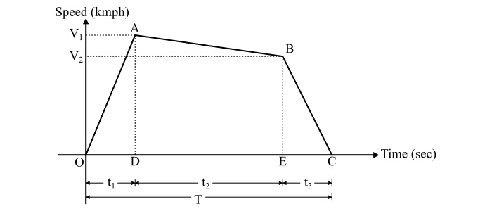
Electric Traction: Quadrilateral Speed Time Curve

For urban and suburban services, the simplified quadrilateral speed-time curve of electric traction is shown in the figure.

Let,

• $\alpha$ = Acceleration in kmphps

• $\beta$ = Braking retardation in kmphps

• $\beta_{c}$ = Coasting retardation in kmphps

• V₁ = Maximum speed at the end of acceleration in kmph

• V₂ = Speed at the end of coasting in kmph

• T = Total time of run in seconds

• t₁ = Acceleration time in seconds

• t₂ = Coasting time in seconds

• t₃ = Braking time in seconds

• D = Total distance travell in km

Therefore, the time of acceleration is given by,

$$\mathrm{\mathit{t_{\mathrm{1}}}\:=\:\frac{\mathit{V_{\mathrm{1}}}}{\alpha } }$$

The time of coasting is given by,

$$\mathrm{\mathit{t_{\mathrm{2}}}\:=\:\frac{\mathit{V_{\mathrm{1}}}-\mathit{V_{\mathrm{2}}}}{\beta_{c} } \:\:\:\cdot \cdot \cdot \mathrm{\left ( \mathrm{1} \right )}}$$

The time of braking is given by,

$$\mathrm{\mathit{t_{\mathrm{3}}}\:=\:\frac{\mathit{V_{\mathrm{2}}}}{\beta }}$$

Now, the total distance travelled in km is

$$\mathrm{\mathit{D}\:=\:\mathrm{distance\: travelled\: during \:acceleration\:+\:distance\: travelled\: during \:coasting\:+\:distance\: travelled\: during \:retardation}}$$

$$\mathrm{\Rightarrow \mathit{D}\:=\:\mathrm{Area\: of \:\bigtriangleup OAD\:+\:Area \:of\: quadrilateral\: DABE\:+\:Area\: of \:\bigtriangleup CEB}}$$

$$\mathrm{\Rightarrow \mathit{D}\:=\:\mathrm{\left (\frac{1}{2}\times \mathit{V_{\mathrm{1}}}\times \frac{\mathit{t_{\mathrm{1}}}}{3600} \right )}\:+\:\mathrm{\left ( \frac{\mathit{V_{\mathrm{1}}}+\mathit{V_{\mathrm{2}}}}{2}\times \frac{\mathit{t_{\mathrm{2}}}}{3600} \right )}\:+\:\mathrm{\left (\frac{1}{2}\times \mathit{V_{\mathrm{2}}}\times \frac{\mathit{t_{\mathrm{3}}}}{3600} \right )}}$$

$$\mathrm{\Rightarrow \mathit{D}\:=\:\frac{\mathit{V_{\mathrm{1}}\mathit{t_{\mathrm{1}}}}}{7200}\:+\:\frac{\mathit{V_{\mathrm{1}}\mathit{t_{\mathrm{2}}}}}{7200}\:+\:\frac{\mathit{V_{\mathrm{2}}\mathit{t_{\mathrm{2}}}}}{7200}\:+\:\frac{\mathit{V_{\mathrm{2}}\mathit{t_{\mathrm{3}}}}}{7200}}$$

$$\mathrm{\Rightarrow \mathit{D}\:=\:\frac{\mathit{V_{\mathrm{1}}}}{7200}\mathrm{\left ( \mathit{t_{\mathrm{1}}+\mathit{t_{\mathrm{2}}}} \right )}\:+\:\frac{\mathit{V_{\mathrm{2}}}}{7200}\mathrm{\left ( \mathit{t_{\mathrm{2}}+\mathit{t_{\mathrm{3}}}} \right )}}$$

$$\mathrm{\because \mathit{T}\:=\:\mathit{t_{\mathrm{1}}}\:+\:\mathit{t_{\mathrm{2}}}\:+\:\mathit{t_{\mathrm{3}}}}$$

$$\mathrm{\Rightarrow \mathit{t_{\mathrm{1}}}\:+\:\mathit{t_{\mathrm{2}}}\:=\:\mathit{T-\mathit{t_{\mathrm{3}}}}\:\mathrm{and}\:\mathit{t_{\mathrm{2}}}\:+\:\mathit{t_{\mathrm{3}}}\:=\:\mathit{T-\mathit{t_{\mathrm{1}}}}}$$

$$\mathrm{\therefore \mathit{D}\:=\:\frac{\mathit{V_{\mathrm{1}}}}{7200}\mathrm{\left ( \mathit{T-\mathit{t_{\mathrm{3}}}} \right )}\:+\:\frac{\mathit{V_{\mathrm{2}}}}{7200}\mathrm{\left ( \mathit{T-\mathit{t_{\mathrm{1}}}} \right )}}$$

$$\mathrm{\Rightarrow \mathit{D}\:=\:\frac{\mathit{T}}{7200}\mathrm{\left ( \mathit{V_{\mathrm{1}}+\mathit{V_{\mathrm{2}}}} \right )}\:-\:\frac{\mathit{V_{\mathrm{1}}t_{\mathrm{3}}}}{7200}\:-\:\frac{\mathit{V_{\mathrm{2}}t_{\mathrm{1}}}}{7200}}$$

On substituting the values of t₁ and t₃, we get,

$$\mathrm{\Rightarrow \mathit{D}\:=\:\frac{\mathit{T}}{7200}\mathrm{\left ( \mathit{V_{\mathrm{1}}+\mathit{V_{\mathrm{2}}}} \right )}\:-\frac{\mathit{V_{\mathrm{1}}\mathit{V_{\mathrm{2}}}}}{7200\beta }\:-\:\frac{\mathit{V_{\mathrm{1}}\mathit{V_{\mathrm{2}}}}}{7200\alpha }}$$

$$\mathrm{\Rightarrow 7200\mathit{D}\:=\:\mathit{T}\mathrm{\left ( \mathit{V_{\mathrm{1}}+\mathit{V_{\mathrm{2}}}} \right )}-\mathit{V_{\mathrm{1}}\mathit{V_{\mathrm{2}}}}\mathrm{\left ( \frac{1}{\alpha }\:+\:\frac{1}{\beta } \right )}\:\:\:\cdot \cdot \cdot \mathrm{\left ( 2 \right )}}$$

Now, by rearranging the equation (1), we get,

$$\mathrm{\mathit{V_{\mathrm{2}}}\:=\:\mathit{V_{\mathrm{1}}}-\beta _{c}\mathit{t_{\mathrm{2}}}}$$

$$\mathrm{\Rightarrow \mathit{V_{\mathrm{2}}}\:=\:\mathit{V_{\mathrm{1}}}-\beta _{c}\mathrm{\left ( \mathit{T-\mathit{t_{\mathrm{1}}-t_{\mathrm{3}}}} \right )}\:=\:\mathit{V_{\mathrm{1}}}-\beta _{c}\mathrm{\left ( \mathit{T-\frac{\mathit{V_{\mathrm{1}}}}{\alpha }-\frac{\mathit{V_{\mathrm{2}}}}{\beta }} \right )}}$$

$$\mathrm{\Rightarrow \mathit{V_{\mathrm{2}}}-\frac{\beta _{c}\mathit{V_{\mathrm{2}}}}{\beta }\:=\:\mathit{V_{\mathrm{1}}}-\beta _{c}\mathrm{\left ( \mathit{T-\frac{\mathit{V_{\mathrm{1}}}}{\alpha }} \right )}}$$

$$\mathrm{\therefore \mathit{V_{\mathrm{2}}}\:=\:\frac{\mathit{V_{\mathrm{1}}}-\beta _{c}\mathit{T}+\frac{\beta _{c}}{\alpha }\mathit{V_{\mathrm{1}}}}{1-\frac{\beta _{c}}{\beta }}\:\:\:\cdot \cdot \cdot \mathrm{\left ( 3 \right )}}$$

Hence, by solving the equations (2) and (3), the values of D, V1 and V2 etc. can be determined.

Numerical Example

A train is required to run between two stations 1.5 km apart at an average speed of 50 kmph. The run is to be made to a simplified quadrilateral speed-time curve. If the maximum speed is to be limited to 60 kmph, acceleration to 2 kmphps and coasting and braking retardations to 0.15 kmphps and 3 kmphps respectively and the speed of the train before applying the brakes is 48 kmph. Determine the duration of acceleration, coasting and braking.

Solution

Given,

• Distance of run,D = 1.5 km

• Average speed,V_α = 50 kmph

• maximum speed,V₁ = 60 kmph

• Speed at the end of coasting,V₂ = 48 kmph

• Acceleration,α = 2 kmphps

• Coasting retardation,β_c = 0.15 kmphps

• Braking retardation,β = 3 kmphps

Therefore, the duration of acceleration is,

$$\mathrm{\mathit{t_{\mathrm{1}}}\:=\:\frac{\mathit{V_{\mathrm{1}}}}{\alpha }\:=\:\frac{60}{2}\:=\:30 \:\mathrm{seconds}}$$

The duration of coasting is,

$$\mathrm{\mathit{t_{\mathrm{2}}}\:=\:\frac{\mathit{V_{\mathrm{1}}}-\mathit{V_{\mathrm{2}}}}{\beta_{c} }\:=\:\frac{60-48}{0.15}\:=\:80 \:\mathrm{seconds}}$$

And theduration of braking is,

$$\mathrm{\mathit{t_{\mathrm{3}}}\:=\:\frac{\mathit{V_{\mathrm{3}}}}{\beta }\:=\:\frac{48}{3}\:=\:16 \:\mathrm{seconds}}$$