Chainer - Quick Guide

---

---

Chainer - Introduction

Chainer is a deep learning framework that prioritizes flexibility and ease of use. One of its standout features is the define-by-run approach where the computational graph is generated dynamically as the code runs rather than being defined upfront. This approach contrasts with more rigid frameworks and allows for greater adaptability, particularly when developing complex models like recurrent neural networks (RNNs) or models that involve conditional operations.

The Chainer Framework is designed to be accessible to both novice and experienced developers, Chainer integrates smoothly with NumPy and efficiently leverages GPU resources for handling large-scale computations. Its ecosystem is robust by offering extensions such as ChainerMN for distributed learning, ChainerRL for reinforcement learning and ChainerCV for computer vision tasks by making it suitable for a wide array of applications.

Chainer's framework is combination of flexibility and a strong ecosystem has made it a popular choice in academic research and industry, especially in Japan where it was first developed. Despite the rise of other frameworks the Chainer remains a powerful tool for those who need a dynamic and user-friendly platform for deep learning.

Key Features of Chainer

Following are the Key features of the Chainer Frame −

• Dynamic Graph Construction (Define-by-Run): When compared to static frameworks, Chainer constructs its computational graph on-the-fly as operations are executed. This dynamic approach enhances flexibility by making it easier to implement complex models such as those involving loops or conditional statements.
• Integration with NumPy: Chainer seamlessly integrates with NumPy by allowing users to leverage familiar array operations and simplifying the process of transitioning from scientific computing to deep learning.
• GPU Optimization: This framework is designed to make efficient use of GPUs which accelerates the training of large-scale models and computations which are critical for handling complex neural networks and extensive datasets.
• Comprehensive Ecosystem: Chainer's ecosystem includes various tools and extensions such as ChainerMN for distributed computing, ChainerRL for reinforcement learning and ChainerCV for tasks in computer vision which broaden its applicability across different fields.
• Customizability: Users can easily create custom components such as layers and loss functions by providing extensive control over the design and behavior of neural networks.

Advantages of Chainer

The Chainer Frame work has many advantages, which helps the users to work effectively. Let's see them in detail as below −

• Adaptability: The Chainer Frame work is more ability to dynamically build and modify the computational graph as needed makes Chainer highly adaptable, facilitating experimentation with novel architectures and models.
• Ease of Use: Chainer's straightforward design and its compatibility with NumPy make it accessible for users at various experience levels, from beginners to advanced practitioners.
• Effective GPU Utilization: By harnessing GPU power the Chainer efficiently manages the demands of training deep learning models by improving performance and reducing computation time.
• Strong Community and Support:Chainer benefits from an active user community and ongoing support particularly in Japan, which helps in troubleshooting and continuously improving the framework.
• Versatile Applications: The Chainer's Framework extensive range of extensions and tools allows Chainer to be used effectively across different domains, from basic machine learning tasks to complex deep learning applications.

Applications of Chainer in Machine Learning

Chainer Framework offers a versatile platform for a wide range of machine learning applications which makes it a powerful tool for developing and deploying advanced models across various domains.

• Neural Network Construction: Chainer is well-suited for developing various neural network architectures such as feedforward, convolutional and recurrent networks. Its dynamic graph creation process allows for flexible and efficient model design which is even for complex structures.
• Computer Vision: Chainer excels in computer vision tasks, particularly with the ChainerCV extension which supports image classification, object detection and segmentation. It leverages deep learning models to effectively process and analyze visual data.
• Natural Language Processing (NLP): Chainer's adaptability makes it ideal for NLP applications such as text classification, language modeling and translation. It supports advanced models like transformers and RNNs, crucial for understanding and generating human language.
• Reinforcement Learning: The ChainerRL extension equips Chainer to handle reinforcement learning tasks by enabling the development of algorithms where agents learn to make decisions in various environments, utilizing techniques such as Q-learning and policy gradients.
• Generative Modeling: Chainer is capable of building and training generative models such as GANs and VAEs. These models are used to create synthetic data that closely mimics real-world datasets.
• Time Series Analysis: With the support for RNNs and LSTMs, Chainer is effective in time series analysis by making it suitable for forecasting in fields like finance and weather prediction, where data sequences are key.
• Automated Machine Learning (AutoML): Chainer is also used in AutoML tasks, automating the selection of models and tuning of hyperparameters. This automation streamlines the machine learning workflow by optimizing the process for better results.
• Distributed Training: ChainerMN allows Chainer to perform distributed training across multiple GPUs or nodes by making it possible to scale machine learning models efficiently and handle large-scale datasets.
• Research and Development: Chainer is highly valued in research settings for its flexibility and ease of experimentation by enabling rapid prototyping and testing of new machine learning concepts and algorithms.

Chainer - Installation

Chainer is a versatile deep learning framework that enables dynamic graph construction by making it suitable for a wide range of machine learning tasks. Whether we are new to deep learning or an experienced developer, setting up Chainer on our system is a simple process.

Installation and Setup of Chainer

Let's go through the steps for installation and setup which ensures us fully equipped to begin building deep learning models with Chainer −

Prerequisites

Before we are installing Chainer, we should ensure that our system meets the following prerequisites −

Python

Chainer supports Python 3.5 and above. It's recommended to use Python 3.7 or later for the best compatibility and performance.

We should ensure Python is installed on our system. We can download the latest version from the official Python Website. We Python already installed in our system we can verify our installation by running the following code −

python --version

Following is the python version installed in the system −

Python 3.12.5

Pip

Pip is the package manager used to install Chainer and its dependencies in our working environment. Generally Pip comes with Python, but we can install and upgrade it with the help of below code −

python -m ensurepip --upgrade

Below is the output of the above code execution −

Defaulting to user installation because normal site-packages is not writeable
Looking in links: c:\Users\91970\AppData\Local\Temp\tmpttbcugpx
Requirement already satisfied: pip in c:\program files\windowsapps\pythonsoftwarefoundation.python.3.12_3.12.1520.0_x64__qbz5n2kfra8p0\lib\site-packages (24.2)

After installation and upgradation we can check the version of the installed pip by executing the below code −

pip --version

Following is the version of the pip installed in the system −

pip 24.2 from C:\Program Files\WindowsApps\PythonSoftwareFoundation.Python.3.12_3.12.1520.0_x64__qbz5n2kfra8p0\Lib\site-packages\pip (python 3.12)

Installing Chainer

Once we've met the prerequisites we can proceed with installing Chainer. The installation process is straightforward and can be +one using two methods such as pip and Pythons package manager. Here's how we can do it −

Installing Chainer with CPU Support

-

If we want to install Chainer without GPU support, we can install it directly with the help of pip. The following command can be used to install the latest version of Chainer along with the necessary dependencies. This is suitable for systems that don't need the GPU acceleration −

pip install chainer

Below is the output of installation of Chainer Framework −

Defaulting to user installation because normal site-packages is not writeable
Requirement already satisfied: chainer in c:\users\91970\appdata\local\packages\pythonsoftwarefoundation.python.3.12_qbz5n2kfra8p0\localcache\local-packages\python312\site-packages (7.8.1)
............................
............................
............................
Requirement already satisfied: six>=1.9.0 in c:\users\91970\appdata\local\packages\pythonsoftwarefoundation.python.3.12_qbz5n2kfra8p0\localcache\local-packages\python312\site-packages (from chainer) (1.16.0)

Installing Chainer with GPU Support

If we want to take advantage of GPU acceleration we need to install Chainer with CUDA support. The version of Chainer we install should match the version of CUDA installed on our system.

We can install the different versions of chainer by replacing the version number with the one corresponding to our installed CUDA version.

For CUDA 9.0

If we want to install Chainer with the help of CUDA 9.0 support with the help of below command. This command ensures that Chainer is installed along with the necessary dependencies to utilize GPU acceleration with CUDA 9.0.

pip install chainer[cuda90]

For CUDA 10.0

Here we can use the below command to install the chainer, which tells pip to install Chainer along with the libraries required for CUDA 10.0 support. The 100 corresponds to CUDA version 10.0 −

pip install chainer[cuda100]

For CUDA 10.1

Following command specifies that Chainer should be installed with the libraries required to support CUDA 10.1. The 101 corresponds to CUDA version 10.1.

pip install chainer[cuda101]

For CUDA 11.0 and later

Below is the command specifies that Chainer should be installed with support for CUDA 11.0. The 110 corresponds to CUDA version 11.0.

pip install chainer[cuda110]

Verifying the Installation

After installing Chainer it's important to ensure that the installation was successful and that Chainer is ready to use. We can test the installation by running the python script with the code as mentioned below −

import chainer
print(chainer.__version__)

Below is the version of the Chainer framework installed in the system −

7.8.1

Installing Additional Extensions

Chainer comes with several optional extensions that are useful for specific tasks. Depending on our project needs we might have to install as follows −

• ChainerMN: A tool for distributed deep learning by enabling model training across multiple GPUs or nodes.

  pip install chainermn
  

• ChainerRL: A suite designed for reinforcement learning by offering resources to develop and train reinforcement learning algorithms.

  pip install chainerrl
  

• ChainerCV: For computer vision applications which includes tools and models for tasks like object detection and image segmentation.

  pip install chainercv
  

Setting up the Virtual Environment

Using a virtual environment is recommended to isolate our Chainer installation and its dependencies from other Python projects. To avoid conflicts with other Python packages, it's a good idea to use a virtual environment. Below is the code of installing the virtual environment −

pip install virtualenv

Now after installing, we can create the virtual environment with the help of below code −

virtualenv chainer_env

Here we are activating the virtual environment by executing the below code on windows platform −

chainer_env\Scripts\activate

If we want to activate the virtual environment in the MacOs/Linux, then we have to execute the below code −

source chainer_env/bin/activate

Now install the chainer framework in the virtual environment with the below code −

pip install chainer

Troubleshooting Common Installation Issues

• CUDA Compatibility: Ensure that the version of CUDA installed on our system matches the one specified during the Chainer installation. Mismatches can cause runtime errors.
• Dependency Conflicts: If we encounter issues with dependencies then try updating pip with pip install --upgrade pip and reinstalling Chainer.

By following all the above mentioned steps the Chainer will be successfully installed on our system by allowing us to start developing and training deep learning models. Whether were working with CPUs or GPUs, Chainer provides the flexibility and power we need for a wide range of machine learning tasks.

Chainer - Neural Networks

Neural networks are computational models inspired by the human brain's structure and function. They consist of interconnected layers of nodes i.e. neurons, where each node processes input data and passes the result to the next layer. The network learns to perform tasks by adjusting the weights of these connections based on the error of its predictions.

This learning process is often called training which enables neural networks to identify patterns, classify data and make predictions. They are widely used in machine learning for tasks such as image recognition, natural language processing and more.

Structure of a Neural Network

A neural network is a computational model that mimics the way neurons in the human brain work. It is composed of layers of nodes known as neurons, which are connected by edges or weights. A typical neural network has an input layer, one or more hidden layers and an output layer. Following is the detailed structure of a Neural network −

Input Layer

The Input layer is the first layer in a neural network and serves as the entry point for the data that will be processed by the network. It doesnt perform any computations rather, it passes the data directly to the next layer in the network.

Following are the key characteristics of the input layer −

• Nodes/Neurons: Each node in the input layer represents a single feature from the input data. For example if we have an image with 28x28 pixels then the input layer would have 784 nodes i.e. one for each pixel.
• Data Representation: The input data is often normalized or standardized before being fed into the input layer to ensure that all features have the same scale which helps in improving the performance of the neural network.
• No Activation Function: Unlike the hidden and output layers the input layer does not apply an activation function. Its primary role is to distribute the raw input features to the subsequent layers for further processing.

Hidden layers

Hidden layers are situated between the input layer and the output layer in a neural network. They are termed "hidden" because their outputs are not directly visible in the input data or the final output predictions.

The primary role of these layers is to process and transform the data through multiple stages by enabling the network to learn complex patterns and features. This transformation is achieved through weighted connections and non-linear activation functions which allow the network to capture intricate relationships within the data.

Following are the key characteristics of the input layer −

• Nodes/Neurons: Each hidden layer consists of multiple neurons which apply weights to the inputs they receive and pass the results through an activation function. The number of neurons and layers can vary depending on the complexity of the task.
• Weights and Biases: Each neuron in a hidden layer has associated weights and biases which are adjusted during the training process. These parameters help the network learn the relationships and patterns in the data.
• Activation Function: Hidden layers typically use activation functions to introduce non-linearity into the model. Common activation functions are mentioned below −
  • ReLU (Rectified Linear Unit): ReLU()=max(0,)
  • Sigmoid: ()=1/(1+e^-x)
  • Tanh (Hyperbolic Tangent): tanh(x) = (e^x - e^-x)/(e^x + e^-x)
  • Leaky ReLU: Leaky ReLU(x) = max(0.01x,x)
• Learning and Feature Extraction: Hidden layers are where most of the learning occurs. They transform the input data into representations that are more suitable for the task at hand. Each successive hidden layer builds on the features extracted by the previous layers which allows the network to learn complex patterns.
• Depth and Complexity: The number of hidden layers and neurons in each layer determine the depth and complexity of the network. More hidden layers and neurons generally allow the network to learn more intricate patterns but also increase the risk of overfitting and require more computational resources.

Output Layer

The output layer is the final layer in a neural network that produces the network's predictions or results. This layer directly generates the output corresponding to the given input data based on the transformations applied by the preceding hidden layers.

The number of neurons in the output layer typically matches the number of classes or continuous values the model is expected to predict. The output is often passed through an activation function such as softmax for classification tasks to provide a probability distribution over the possible classes.

Following are the key characteristics of the output layer −

• Nodes/Neurons: The number of neurons in the output layer corresponds to the number of classes or target variables in the problem. For example if in a binary classification problem then there would be one neuron or two neurons in some setups. In a multi-class classification problem with 10 classes then there would be 10 neurons.
• Activation Function: These in the output layer play a crucial role in shaping the final output of a neural network by making them appropriate for the specific type of prediction task such as classification, regression, etc. The choice of activation function directly influences the interpretation of the network's predictions. Common activation functions are mentioned below −
  • Classification Tasks: Commonly use the softmax activation function for multi-class classification which converts the output to a probability distribution over the classes or sigmoid for binary classification.
  • Regression Tasks: Typically use a linear activation function as the goal is to predict a continuous value rather than a class.
  • Tanh (Hyperbolic Tangent): tanh(x) = (e^x - e^-x)/(e^x + e^-x)
  • Leaky ReLU: Leaky ReLU(x) = max(0.01x,x)
• Output: The output layer delivers the final result of the network which may be a probability, a class label or a continuous value which depends on the type of task. In classification tasks the neuron with the highest output value typically indicates the predicted class.

Types of Neural Networks

Neural networks come in various architectures with each tailored to specific types of data and tasks. Here's a detailed overview of the primary types of neural networks −

Feedforward Neural Networks (FNNs)

Feedforward Neural Networks (FNNs) are a fundamental class of artificial neural networks characterized by their unidirectional flow of information. In these networks the data travels in a single direction i.e. from the input layer, through any hidden layers and finally to the output layer. This architecture ensures that there are no cycles or loops in the connections between nodes (neurons).

Following are the key features of FNNs −

• Architecture: FNNs are composed of three principal layers as mentioned below −
  • Input Layer: This layer receives the initial data features.
  • Hidden Layers: Intermediate layers that process the data and extract relevant features. Neurons in these layers apply activation functions to their inputs.
  • Output Layer: This final layer produces the network's output which can be a classification label, probability or a continuous value.
• Forward Propagation: Data moves through the network from the input layer to the output layer. Each neuron processes its input and transmits the result to the next layer.
• Activation Functions: These functions introduce non-linearity into the network by allowing it to model more complex relationships. Typical activation functions include ReLU, sigmoid and tanh.
• Training: FNNs are trained using methods like backpropagation and gradient descent. This process involves updating the network's weights to reduce the error between the predicted and actual outcomes.
• Applications: FNNs are employed in various fields such as image recognition, speech processing and regression analysis.

Convolutional Neural Networks (CNNs)

Convolutional Neural Networks (CNNs) are a specialized type of neural network designed to process data with a grid-like topology such as images. They are particularly effective for tasks involving spatial hierarchies and patterns such as image and video recognition.

Following are the key features of the CNNs −

• Architecture: CNNs are composed of three principal layers as defined below −
  • Convolutional Layers: These layers apply convolutional filters to the input data. Each filter scans the input to detect specific features such as edges or textures. The convolution operation produces feature maps that highlight the presence of these features.
  • Pooling Layers: This layer is also known as subsampling or downsampling layers. The pooling layers reduce the spatial dimensions of feature maps while retaining essential information. Common pooling operations include max pooling which selects the maximum value and average pooling which computes the average value.
  • Fully Connected Layers: After several convolutional and pooling layers, the high-level feature maps are flattened into a one-dimensional vector and passed through fully connected layers. These layers perform the final classification or regression based on the extracted features.
• Forward Propagation: In CNNs the data moves through the network in a series of convolutional, pooling and fully connected layers. Each convolutional layer detects features while pooling layers reduce dimensionality and fully connected layers make final predictions.
• Activation Functions: CNNs use activation functions like ReLU (Rectified Linear Unit) to introduce non-linearity which helps the network learn complex patterns. Other activation functions like sigmoid and tanh may also be used depending on the task.
• Training: CNNs are trained using techniques such as backpropagation and optimization algorithms like stochastic gradient descent (SGD). During training the network learns the optimal values for convolutional filters and weights to minimize the error between predicted and actual outcomes.
• Applications: CNNs are widely used in computer vision tasks such as image classification, object detection and image segmentation. They are also applied in fields like medical image analysis and autonomous driving where spatial patterns and hierarchies are crucial.

Long Short-Term Memory Networks (LSTMs)

LSTMs are a type of Recurrent Neural Network (RNN) designed to address specific challenges in learning from sequential data, particularly the problems of long-term dependencies and vanishing gradients. They enhance the basic RNN architecture by introducing specialized components that allow them to retain information over extended periods.

Following are the key features of the LSTMs −

• Architecture: Below are the details of the architechure of LSTMs Networks −
  • Cell State: LSTMs include a cell state that acts as a memory unit by carrying information across different time steps. This state is updated and maintained through the network by allowing it to keep relevant information from previous inputs.
  • Gates: LSTMs use gates to control the flow of information into and out of the cell state. These gates include −
    • Forget Gate: This gate determines which information from the cell state should be discarded.
    • Input Gate: This controls the addition of new information to the cell state.
    • Output Gate: This gate regulates what part of the cell state should be outputted and passed to the next time step.
• Hidden State:In addition to the cell state, the LSTMs maintain a hidden state that represents the output of the network at each time step. The hidden state is updated based on the cell state and influences the predictions made by the network.
• Forward Propagation: During forward propagation the LSTMs process the input data step-by-step by updating the cell state and hidden state as they go. The gates regulate the information flow ensuring that relevant information is preserved while irrelevant information is filtered out. The final output at each time step is derived from the hidden state which incorporates information from the cell state.
• Activation Functions: LSTMs use activation functions such as sigmoid and tanh to manage the gating mechanisms and update the cell and hidden states. The sigmoid function is used to compute the gates while tanh is applied to regulate the values within the cell state.
• Training: LSTMs are trained using backpropagation through time (BPTT) which are similar to other RNNs. This process involves unfolding the network across time steps and applying backpropagation to update the weights based on the error between the predicted and actual outputs. LSTMs mitigate issues like vanishing gradients by effectively managing long-term dependencies by making them more suitable for tasks requiring memory of past inputs.
• Applications: LSTMs are particularly useful for tasks involving complex sequences and long-term dependencies including: −
  • Natural Language Processing (NLP): For tasks such as language modeling, machine translation, and text generation, where understanding context over long sequences is crucial.
  • Time Series Forecasting: Predicting future values in data with long-term trends such as stock market analysis or weather prediction.
  • Speech Recognition: Converting spoken language into text by analyzing and retaining information from audio sequences over time.

Recurrent Neural Networks (RNNs)

Recurrent Neural Networks (RNNs) are specialized for handling sequential data by using internal memory through hidden states. This capability makes them ideal for tasks where understanding the sequence or context is essential such as in language modeling and time series prediction.

Following are the key features of the RNNs −

• Architecture: RNNs are composed of two principal layers which are given below −
  • Recurrent Layers: RNNs are characterized by their looping connections within the network by enabling them to maintain and update a memory of past inputs via a hidden state. This feature allows the network to use information from previous steps to influence current and future predictions.
  • Hidden State: This serves as the network's internal memory which is updated at each time step. It retains information from earlier inputs and impacts the processing of subsequent inputs.
• Forward Propagation: Data in RNNs progresses sequentially through the network. At each time step the network processes the current input, updates the hidden state based on the previous inputs and generates an output. The updated hidden state is then used for processing the next input.
• Activation Functions: To model complex patterns and introduce non-linearity the RNNs use activation functions such as tanh or ReLU. Advanced RNN variants like Long Short-Term Memory (LSTM) networks and Gated Recurrent Units (GRUs) include additional mechanisms to better manage long-term dependencies and address challenges such as vanishing gradients.
• Training: RNNs are trained through a method called backpropagation through time (BPTT). This involves unfolding the network across time steps and applying backpropagation to adjust weights based on the discrepancy between predicted and actual outputs. Training RNNs can be difficult due to issues like vanishing gradients which are often mitigated by using advanced RNN architectures.
• Applications: RNNs are particularly effective for tasks involving sequential data such as −
• Natural Language Processing (NLP): Applications such as text generation, machine translation, and sentiment analysis.
• Time Series Forecasting: Predicting future values in sequences, such as stock prices or weather conditions.
• Speech Recognition: Converting spoken language into text by analyzing sequences of audio data.

Generative Adversarial Networks (GANs)

Generative Adversarial Networks (GANs) are a class of machine learning frameworks designed to generate realistic data samples. GANs consist of two neural networks one is a generator and other is a discriminator which are trained together in a competitive setting. This adversarial process allows GANs to produce data that closely mimics real-world data.

Following are the key features of the GANs −

• Architecture: GANs are mainly consists of two networks in their architecture −
  • Generator: The generator's role is to create fake data samples from random noise. It learns to map this noise to data distributions similar to the real data. The generator's goal is to create data that is indistinguishable from real data in the eyes of the discriminator.
  • Discriminator: The discriminator's role is to distinguish between real data (from the actual dataset) and fake data (produced by the generator). It outputs a probability indicating whether a given sample is real or fake. The discriminator aims to correctly classify the real and fake samples.
• Adversarial Process: The process of training the Generators and Discriminators at the same time is known as Adversarial Process. Let's see the important processes in GANs −
• Generator Training: The generator creates a batch of fake data samples and sends them to the discriminator and trying to fool it into thinking they are real.
• Discriminator Training: The discriminator receives both real data and fake data from the generator and it tries to correctly identify which is fake and real data.
• Loss Functions: The generator's loss is based on how well it can fool the discriminator while the discriminator's loss is based on how accurately it can distinguish real from fake data. The networks are updated alternately with the generator trying to minimize its loss and the discriminator trying to maximize its accuracy.
• Convergence: The training process continues until the generator produces data so realistic that the discriminator can no longer distinguish between real and fake samples with high accuracy. At this point the generator has learned to produce outputs that closely resemble the original data distribution.
• Applications: GANs have found extensive applications across multiple domains as mentioned below −
• Image Generation: Producing realistic images, such as generating lifelike human faces or creating original artwork.
• Data Augmentation: Increasing the diversity of training datasets for machine learning models, particularly useful in situations with limited data.
• Style Transfer: Transforming the style of one image to another, like converting a photograph into the style of a specific painting.
• Super-Resolution: Improving the resolution of images by generating detailed, high-resolution outputs from low-resolution inputs.

Autoencoders

Autoencoders are a type of artificial neural network used primarily for unsupervised learning. They are designed to learn efficient representations of data, typically for dimensionality reduction or feature learning. An autoencoder consists of two main parts namely, the encoder and the decoder. The goal is to encode the input data into a lower-dimensional representation (latent space) and then reconstruct the original input from this compressed representation.

Following are the key features of the Autoencoders −

• Architecture: Following are the elements included in the architecture of the Autoencoders −
• Encoder: The encoder compresses the input data into a smaller with latent representation. This process involves mapping the input data to a lower-dimensional space through one or more hidden layers. The encoder's layers use activation functions such as ReLU or sigmoid to transform the input into a compact representation that captures the essential features of the data.
• Latent Space (Bottleneck): The latent space is the compressed with low-dimensional representation of the input data. It acts as a bottleneck that forces the network to focus on the most important features of the data, filtering out noise and redundancy. The size of the latent space determines the degree of compression. A smaller latent space leads to more compression but may lose some information while a larger latent space retains more detail.
• Decoder: The decoder rebuilds the original input data from the latent representation. It has a structure that mirrors the encoder and progressively expanding the compressed data back to its original size. The output layer of the decoder usually employs the same activation function as the input data to produce the final reconstructed output.
• Training: Autoencoders are trained using backpropagation with the objective of minimizing the difference between the original input and the reconstructed output. The loss function used is often mean squared error (MSE) or binary cross-entropy depending on the nature of the input data. The network adjusts its weights during training to learn an efficient encoding that captures the most significant features of the input while being able to reconstruct it accurately.
• Applications: Autoencoders are versatile tools in machine learning which can be applied in various fields such as −
  • Dimensionality Reduction: They help in compressing data by reducing the number of features while retaining crucial information.
  • Anomaly Detection: Autoencoders can identify anomalies by recognizing patterns that differ significantly from normal data typically through reconstruction errors.
  • Data Denoising: They are effective in removing noise from images, signals or other data types.
  • Generative Models: Especially with Variational Autoencoders (VAEs) autoencoders can generate new data samples that closely resemble the original dataset.

Graph Neural Networks (GNNs)

Graph Neural Networks (GNNs) are a specialized type of neural network designed to work with data that is organized in graph structures. In a graph the data is represented as nodes (vertices) connected by edges (relationships).

GNNs utilize this graph-based structure to learn and make predictions by making them particularly useful for tasks where data naturally forms a graph. By effectively capturing the relationships and dependencies between nodes, GNNs excel in tasks that involve complex, interconnected data.

Following are the key features of the GNNs −

• Architecture: Here are the components that are included in the Graph Neural Networks (GNNs)
• Node Representation: Each node in the graph has an initial feature vector representing its attributes. These feature vectors are updated through the network's layers.
• Message Passing: GNNs use a message-passing mechanism where each node exchanges information with its neighboring nodes. This step allows the network to aggregate information from neighboring nodes to update its own representation.
• Aggregation Function: An aggregation function combines the messages received from neighboring nodes. Common aggregation methods include summing, averaging or applying more complex operations.
• Update Function: After aggregation the node's feature vector is updated using a function that often includes neural network layers such as fully connected layers or activation functions.
• Readout Function: The final representation of the graph or nodes can be obtained through a readout function which might aggregate the node features into a global graph representation or compute final predictions.
• Training: The GNNs use below mentioned methods for training purpose −
  • Loss Function: GNNs are trained with loss functions specific to their tasks such as node classification, graph classification or link prediction. The loss function quantifies the difference between the predicted outputs and the actual ground truth.
  • Optimization: The training process involves optimizing the network's weights using gradient-based optimization algorithms. Common methods such as stochastic gradient descent (SGD) and Adam. These methods adjust the weights to minimize the loss by improving the model's accuracy and performance on the given task.
• Applications: Below are the applications where GNNs are used −
• Node Classification: Assigning labels or categories to individual nodes based on their features and the overall graph structure. This is useful for tasks such as identifying types of entities within a network.
• Graph Classification: Categorizing entire graphs into different classes. This can be applied in scenarios like classifying molecules in chemistry or categorizing different types of social networks.
• Link Prediction: Forecasting the likelihood of connections or edges forming between nodes. This is valuable in recommendation systems such as predicting user connections or suggesting products.
• Graph Generation: Creating new graphs or structures from learned patterns. This is beneficial in fields like drug discovery where new molecular structures are proposed based on existing data.
• Social Network Analysis: Evaluating social interactions within a network to identify influential nodes, detect communities or predict social dynamics and trends.

Chainer - Core Components

Chainer is a versatile deep learning framework designed to facilitate the development and training of neural networks with ease. The core components of Chainer provide a robust foundation for building complex models and performing efficient computations.

In chainer the core component the Chain class is used for managing network layers and parameters such as Links and Functions for defining and applying model operations and the Variable class for handling data and gradients.

Additionally the Chainer incorporates powerful Optimizers for updating model parameters, utilities for managing xDataset and DataLoader and a dynamic Computational Graph that supports flexible model architectures. Together all these components enable streamlined model creation, training and optimization by making Chainer a comprehensive tool for deep learning tasks.

Here are the different core components of the Chainer Framework −

Variables

In Chainer the Variable class is a fundamental building block that represents data and its associated gradients during the training of neural networks. A Variable encapsulates not only the data such as inputs, outputs or intermediate computations but also the information required for automatic differentiation which is crucial for backpropagation.

Key Features of Variable

Below are the key features of the variables in the Chainer Framework −

• Data Storage: A Variable holds the data in the form of a multi-dimensional array which is typically a NumPy or CuPy array, depending on whether computations are performed on the CPU or GPU. The data stored in a Variable can be input data, output predictions or any intermediate values computed during the forward pass of the network.
• Gradient Storage: During backpropagation the Chainer computes the gradients of the loss function with respect to each Variable. These gradients are stored within the Variable itself. The grad attribute of a Variable contains the gradient data which is used to update the model parameters during training.
• Automatic Differentiation: Chainer automatically constructs a computational graph as operations are applied to Variable objects. This graph tracks the sequence of operations and dependencies between variables by enabling efficient calculation of gradients during the backward pass. The backward method can be called on a Variable to trigger the computation of gradients throughout the network.
• Device Flexibility: Variable supports both CPU by using NumPy and GPU by using CuPy arrays by making it easy to move computations between devices. Operations on Variable automatically adapt to the device where the data resides.

Example

Following example shows how to use Chainer's Variable class to perform basic operations and calculate gradients via backward propagation −

import chainer
import numpy as np

# Create a Variable with data
x = chainer.Variable(np.array([1.0, 2.0, 3.0], dtype=np.float32))

# Perform operations on Variable
y = x ** 2 + 2 * x + 1

# Print the result
print("Result:", y.data)  # Output: [4. 9. 16.]

# Assume y is a loss and perform backward propagation
y.grad = np.ones_like(y.data)  # Set gradient of y to 1 for backward pass
y.backward()  # Compute gradients

# Print the gradient of x
print("Gradient of x:", x.grad)  # Output: [4. 6. 8.]

Here is the output of the chainer's variable class −

Result: [ 4.  9. 16.]
Gradient of x: [4. 6. 8.]

Functions

In Chainer Functions are operations that are applied to data within a neural network. These functions are essential building blocks that perform mathematical operations, activation functions, loss computations and other transformations on the data as it flows through the network.

Chainer provides a wide range of predefined functions in the chainer.functions module by enabling users to easily build and customize neural networks.

Key functions in Chainer

Activation Functions: These functions in neural networks introduce non-linearity to the model by enabling it to learn complex patterns in the data. They are applied to the output of each layer to determine the final output of the network. Following are the activation functions in chainer −

• ReLU (Rectified Linear Unit): The ReLU outputs are given as input directly if it's positive otherwise it outputs zero. It's widely used in neural networks because it helps mitigate the vanishing gradient problem and is computationally efficient by making it effective for training deep models. The formula for ReLU is given as −

  $$ReLU(x) = max(\theta, x)$$

  The function of ReLU in chainer.functions module is given as F.relu(x).

• sigmoid: This function maps the input to a value between 0 and 1 by making it ideal for binary classification tasks. It provides a smooth gradient which helps in gradient-based optimization but can suffer from the vanishing gradient problem in deep networks. The formula for sigmoid is given as −

  $$Sigmoid(x)=\frac{1}{1+e^{-x}}$$

  The function for Sigmoid in chainer.functionsmodule is given as F.sigmoid(x)

• Tanh (Hyperbolic Tangent): This function in Chainer is employed as an activation function in neural networks. It transforms the input to a value between -1 and 1 by resulting in a zero-centered output. This characteristic can be beneficial during training as it helps to address issues related to non-centered data which potentially improving the convergence of the model. The formula for Tanh is given as −

  $$Tanh(x) = \frac{e^x - e^{-x}}{e^x + e^{-x}}$$

  We have the function F.tanh(x) in chainer.functions module for calculating the Tanh in chainer.

• Leaky ReLU: This is also called as Leaky Rectified Linear Unit function in neural networks is a variant of the standard ReLU activation function. Unlike ReLU which outputs zero for negative input where as Leaky ReLU permits a small, non-zero gradient for negative inputs.

  This adjustment helps prevent the "dying ReLU" problem where neurons become inactive and cease to learn by ensuring that all neurons continue to contribute to the model's learning process. The formula for Leaky ReLU is given as −

  $$Leaky Relu(x) = max(\alpha x, x)$$

  Where, $\alpha$ is a small constant. The chainer.functions module has the function F.leaky_relu(x) to calculate Leaky ReLu in chainer.

• Softmax: This is an activation function typically employed in the output layer of neural networks especially for multi-class classification tasks. It transforms a vector of raw prediction scores (logits) into a probability distribution where each probability is proportional to the exponential of the corresponding input value.

  The probabilities in the output vector sum to 1 by making Softmax ideal for representing the likelihood of each class in a classification problem. The formula for Softmax is given as −

  $$Softmax(x_{i})=\frac{e^{x_{i}}}{\sum_{j} e^{x_{j}}}$$

  The chainer.functions module has the function F.softmax(x) to calculate Softmax in chainer.

Example

Here's an example which shows how to use various activation functions in Chainer within a simple neural network −

import chainer
import chainer.links as L
import chainer.functions as F
import numpy as np

# Define a simple neural network using Chainer's Chain class
class SimpleNN(chainer.Chain):
   def __init__(self):
      super(SimpleNN, self).__init__()
      with self.init_scope():
        # Define layers: two linear layers
        self.l1 = L.Linear(4, 3)  # Input layer with 4 features, hidden layer with 3 units
        self.l2 = L.Linear(3, 2)  # Hidden layer with 3 units, output layer with 2 units
      
   def __call__(self, x):
      # Forward pass using different activation functions
      
      # Apply ReLU activation after the first layer
      h = F.relu(self.l1(x))
      
      # Apply Sigmoid activation after the second layer
      y = F.sigmoid(self.l2(h))
      
      return y
      
# Create a sample input data with 4 features
x = np.array([[0.5, -1.2, 3.3, 0.7]], dtype=np.float32)

# Convert input to Chainer's Variable
x_var = chainer.Variable(x)

# Instantiate the neural network
model = SimpleNN()

# Perform a forward pass
output = model(x_var)

# Print the output
print("Network output after applying ReLU and Sigmoid activations:", output.data)

Here is the output of the Activation functions used in simple neural networks −

Network output after applying ReLU and Sigmoid activations: [[0.20396319 0.7766712 ]]

Chain and ChainList

In Chainer the Chain and ChainList are fundamental classes that facilitate the organization and management of layers and parameters within a neural network. Both Chain and ChainList are derived from chainer.Link the base class responsible for defining model parameters. However they serve different purposes and are used in distinct scenarios. Let's see in detail about the chain and chainlist as follows −

Chain

The Chain class is designed to represent a neural network or a module within a network as a collection of links (layers). When using Chain we can define the network structure by explicitly specifying each layer as an instance variable. This approach is beneficial for networks with a fixed architecture.

We can use Chain when we have a well-defined, fixed network architecture where we want to directly access and organize each layer or component of the model.

Following are the key features of Chain Class −

• Named Components: Layers or links added to a Chain are accessible by name by making it straightforward to reference specific parts of the network.
• Static Architecture: The structure of a Chain is usually defined at initialization and doesn't change dynamically during training or inference.

Example

Following is the example which shows the usage of the Chain class in the Chainer Framework −

import chainer
import chainer.links as L
import chainer.functions as F

# Define a simple neural network using Chain
class SimpleChain(chainer.Chain):
   def __init__(self):
      super(SimpleChain, self).__init__()
      with self.init_scope():
        self.l1 = L.Linear(4, 3)  # Linear layer with 4 inputs and 3 outputs
        self.l2 = L.Linear(3, 2)  # Linear layer with 3 inputs and 2 outputs
      
   def forward(self, x):
      h = F.relu(self.l1(x))  # Apply ReLU after the first layer
      y = self.l2(h)        # No activation after the second layer
      return y
      
# Instantiate the model
model = SimpleChain()
print(model)

Below is the output of the above example −

SimpleChain(
  (l1): Linear(in_size=4, out_size=3, nobias=False),
  (l2): Linear(in_size=3, out_size=2, nobias=False),
)

ChainList

The ChainList class is similar to Chain but instead of defining each layer as an instance variable we can store them in a list-like structure. ChainList is useful when the number of layers or components may vary or when the architecture is dynamic.

We can use the ChainList when we have a model with a variable number of layers or when the network structure can change dynamically. It's also useful for architectures like recurrent networks where the same type of layer is used multiple times.

Following are the key features of ChainList −

• Unordered Components: Layers or links added to a ChainList are accessed by their index rather than by name.
• Flexible Architecture: It is more suitable for cases where the network's structure might change or where layers are handled in a loop or list.

Example

Here is the example which shows how to use the ChainList class in the Chainer Framework −

import chainer
import chainer.links as L
import chainer.functions as F

# Define a neural network using ChainList
class SimpleChainList(chainer.ChainList):
   def __init__(self):
      super(SimpleChainList, self).__init__(
         L.Linear(4, 3),  # Linear layer with 4 inputs and 3 outputs
         L.Linear(3, 2)   # Linear layer with 3 inputs and 2 outputs
      )

   def forward(self, x):
      h = F.relu(self[0](x))  # Apply ReLU after the first layer
      y = self[1](h)        # No activation after the second layer
      return y

# Instantiate the model
model = SimpleChainList()
print(model)

Below is the output of using the ChainList class in Chainer Framework −

SimpleChainList(
  (0): Linear(in_size=4, out_size=3, nobias=False),
  (1): Linear(in_size=3, out_size=2, nobias=False),
)

Optimizers

In Chainer optimizers plays a crucial role in training neural networks by adjusting the model's parameters such as weights and biases which are used to minimize the loss function.

During training, after the gradients of the loss function with respect to the parameters are calculated through back-propagation the optimizers use these gradients to update the parameters in a way that gradually reduces the loss.

Chainer offers a variety of built-in optimizers in which each employing different strategies for parameter updates to suit different types of models and tasks. Following are the key optimizers in Chainer −

SGD (Stochastic Gradient Descent)

The most basic optimizer is SGD updates in which each parameter in the direction of its negative gradient and scaled by a learning rate. It's simple but can be slow to converge.

Often these can be used in simpler or smaller models or as a baseline to compare with more complex optimizers.

The function in chainer to calculate SGD is given as chainer.optimizers.SGD

Example

Here's a simple example of using Stochastic Gradient Descent (SGD) in Chainer to train a basic neural network. We'll use a small dataset which define a neural network model and then apply the SGD optimizer to update the model's parameters during training −

import chainer
import chainer.functions as F
import chainer.links as L
from chainer import Chain
import numpy as np
from chainer import Variable
from chainer import optimizers

class SimpleNN(Chain):
   def __init__(self):
      super(SimpleNN, self).__init__()
      with self.init_scope():
       self.fc1 = L.Linear(None, 100)  # Fully connected layer with 100 units
       self.fc2 = L.Linear(100, 10)   # Output layer with 10 units (e.g., for 10 classes)

   def forward(self, x):
      h = F.relu(self.fc1(x))  # Apply ReLU activation function
      return self.fc2(h)     # Output layer

# Dummy data: 5 samples, each with 50 features
x_data = np.random.rand(5, 50).astype(np.float32)
# Dummy labels: 5 samples, each with 10 classes (one-hot encoded)
y_data = np.random.randint(0, 10, 5).astype(np.int32)

# Convert to Chainer variables
x = Variable(x_data)
y = Variable(y_data)

# Initialize the model
model = SimpleNN()

# Set up SGD optimizer with a learning rate of 0.01
optimizer = optimizers.SGD(lr=0.01)
optimizer.setup(model)
def loss_func(predictions, targets):
   return F.softmax_cross_entropy(predictions, targets)
# Training loop
for epoch in range(10):  # Number of epochs
   # Zero the gradients
   model.cleargrads()
   
   # Forward pass
   predictions = model(x)
   
   # Calculate loss
   loss = loss_func(predictions, y)
   
   # Backward pass
   loss.backward()
   
   # Update parameters
   optimizer.update()
   
   # Print loss
   print(f'Epoch {epoch + 1}, Loss: {loss.data}')

Following is the output of the SGD optimizer −

Epoch 1, Loss: 2.3100974559783936
Epoch 2, Loss: 2.233552932739258
Epoch 3, Loss: 2.1598660945892334
Epoch 4, Loss: 2.0888497829437256
Epoch 5, Loss: 2.020642042160034
Epoch 6, Loss: 1.9552147388458252
Epoch 7, Loss: 1.8926388025283813
Epoch 8, Loss: 1.8325523138046265
Epoch 9, Loss: 1.7749309539794922
Epoch 10, Loss: 1.7194255590438843

Momentum SGD

The Momentum SGDis an extension of SGD that includes momentum which helps to accelerate gradients vectors in the right directions by leading to faster converging. It accumulates a velocity vector in the direction of the gradient.

This is suitable for models where vanilla SGD struggles to converge. We have the function called chainer.optimizers.MomentumSGD to perform the Momentum SGD optimization.

Momentum Term: Adds a fraction of the previous gradient update to the current update. This helps to accelerate gradients vectors in the right directions and dampen oscillations.

Formula: The update rule for parameters with momentum is given as −

$$v_{t} = \beta v_{t-1} + (1 - \beta) \nabla L(\theta)$$ $$\theta = \theta-\alpha v_{t}$$

Where −

• $v_{t}$ is the velocity (or accumulated gradient)
• $\beta$ is the momentum coefficient (typically around 0.9)
• $\alpha$ is the learning rate
• $\nabla L(\theta)$ is the gradient of the loss function with respect to the parameters.

Example

Here's a basic example of how to use the Momentum SGD optimizer with a simple neural network in Chainer −

import chainer
import chainer.functions as F
import chainer.links as L
from chainer import Chain
from chainer import optimizers
import numpy as np
from chainer import Variable

class SimpleNN(Chain):
   def __init__(self):
      super(SimpleNN, self).__init__()
      with self.init_scope():
       self.fc1 = L.Linear(None, 100)  # Fully connected layer with 100 units
       self.fc2 = L.Linear(100, 10)   # Output layer with 10 units (e.g., for 10 classes)

   def forward(self, x):
      h = F.relu(self.fc1(x))  # Apply ReLU activation function
      return self.fc2(h)     # Output layer


# Dummy data: 5 samples, each with 50 features
x_data = np.random.rand(5, 50).astype(np.float32)
# Dummy labels: 5 samples, each with 10 classes (one-hot encoded)
y_data = np.random.randint(0, 10, 5).astype(np.int32)

# Convert to Chainer variables
x = Variable(x_data)
y = Variable(y_data)


# Initialize the model
model = SimpleNN()

# Set up Momentum SGD optimizer with a learning rate of 0.01 and momentum of 0.9
optimizer = optimizers.MomentumSGD(lr=0.01, momentum=0.9)
optimizer.setup(model)
def loss_func(predictions, targets):
   return F.softmax_cross_entropy(predictions, targets)
# Training loop
for epoch in range(10):  # Number of epochs
   # Zero the gradients
   model.cleargrads()
   
   # Forward pass
   predictions = model(x)
   
   # Calculate loss
   loss = loss_func(predictions, y)
   
   # Backward pass
   loss.backward()
   
   # Update parameters
   optimizer.update()
   
   # Print loss
   print(f'Epoch {epoch + 1}, Loss: {loss.data}')

Following is the output of the Momentum SGD optimizer −

Epoch 1, Loss: 2.4459869861602783
Epoch 2, Loss: 2.4109833240509033
Epoch 3, Loss: 2.346194267272949
Epoch 4, Loss: 2.25825572013855
Epoch 5, Loss: 2.153470754623413
Epoch 6, Loss: 2.0379838943481445
Epoch 7, Loss: 1.9174035787582397
Epoch 8, Loss: 1.7961997985839844
Epoch 9, Loss: 1.677260398864746
Epoch 10, Loss: 1.5634090900421143

Adam

Adam optimizer combines the advantages of two other extensions of SGD namely AdaGrad, which works well with sparse gradients and RMSProp, which works well in non-stationary settings. Adam maintains a moving average of both the gradients and their squares and updates the parameters based on these averages.

This is often used as the default optimizer due to its robustness and efficiency across a wide range of tasks and models. In chainer we have the function chainer.optimizers.Adam to perform Adam optimization.

Following of the Key features of the Adam optimizer −

• Adaptive Learning Rates: Adam dynamically adjusts the learning rates for each parameter, making it effective across various tasks.
• Moments of Gradients: It calculates the first moment (mean) and second moment (uncentered variance) of gradients to improve optimization.
• Bias Correction: Adam uses bias-correction to address the bias introduced during initialization, particularly early in training.
• Formula: The formula for Adam optimization is given as − $$m_t = \beta_1 m_{t-1} + (1 - \beta_1) \nabla L(\theta)$$ $$v_t = \beta_2 v_{t-1} + (1 - \beta_2) (\nabla L(\theta))^2$$ $$\hat{m}_t = \frac{m_t}{1 - \beta_1^t}$$ $$\hat{v}_t = \frac{v_t}{1 - \beta_2^t}$$ $$\theta = \theta - \frac{\alpha\hat{m}_t}{\sqrt{\hat{v}_t} + \epsilon}$$

  Where, $\alpha$ is the learning rate $\beta 1$ and $\beta 2$ are the decay rates for the moving averages of the gradient and its square, typically 0.9 and 0.999 respectively, ${m_t}$ and ${v_t}$ are the first and second moment estimates and $\epsilon$ is small constant added for numerical stability.

Example

Following is the example which shows how to use the Adam Optimizer in chainer with a neural network −

import chainer
import chainer.functions as F
import chainer.links as L
from chainer import Chain
from chainer import optimizers
import numpy as np
from chainer import Variable

class SimpleNN(Chain):
   def __init__(self):
      super(SimpleNN, self).__init__()
      with self.init_scope():
       self.fc1 = L.Linear(None, 100)  # Fully connected layer with 100 units
       self.fc2 = L.Linear(100, 10)   # Output layer with 10 units (e.g., for 10 classes)

   def forward(self, x):
      h = F.relu(self.fc1(x))  # Apply ReLU activation function
      return self.fc2(h)     # Output layer

# Dummy data: 5 samples, each with 50 features
x_data = np.random.rand(5, 50).astype(np.float32)
# Dummy labels: 5 samples, each with 10 classes (one-hot encoded)
y_data = np.random.randint(0, 10, 5).astype(np.int32)

# Convert to Chainer variables
x = Variable(x_data)
y = Variable(y_data)

# Initialize the model
model = SimpleNN()

# Set up Adam optimizer with default parameters
optimizer = optimizers.Adam()
optimizer.setup(model)
def loss_func(predictions, targets):
   return F.softmax_cross_entropy(predictions, targets)
# Training loop
for epoch in range(10):  # Number of epochs
   # Zero the gradients
   model.cleargrads()
   
   # Forward pass
   predictions = model(x)
   
   # Calculate loss
   loss = loss_func(predictions, y)
   
   # Backward pass
   loss.backward()
   
   # Update parameters
   optimizer.update()
   
   # Print loss
   print(f'Epoch {epoch + 1}, Loss: {loss.data}')

Here is the output of applying the Adam optimizer to a neural network −

Epoch 1, Loss: 2.4677982330322266
Epoch 2, Loss: 2.365001678466797
Epoch 3, Loss: 2.2655398845672607
Epoch 4, Loss: 2.1715924739837646
Epoch 5, Loss: 2.082294464111328
Epoch 6, Loss: 1.9973262548446655
Epoch 7, Loss: 1.9164447784423828
Epoch 8, Loss: 1.8396313190460205
Epoch 9, Loss: 1.7676666975021362
Epoch 10, Loss: 1.7006778717041016

AdaGrad

AdaGrad is also known as Adaptive Gradient Algorithm which is an optimization algorithm that adjusts the learning rate for each parameter based on the accumulated gradient history during training. It is particularly effective for sparse data and scenarios where features vary in frequency or importance.

This is suitable for problems with sparse data and for dealing with models where some parameters require more adjustment than others. The function chainer.optimizers.AdaGrad is used to perfrom AdaGrad optimization in Chainer.

Following are the key features of the AdaGrad Optimizer −

• Adaptive Learning Rates: AdaGrad adjusts the learning rate for each parameter individually based on the cumulative sum of squared gradients. This results in larger updates for infrequent parameters and smaller updates for frequent ones.
• No Need for Learning Rate Tuning: AdaGrad automatically scales the learning rate which often removing the necessity for manual tuning.

Formula: The formula for AdaGrad is given as follows −

$$g_t = \nabla L(\theta)$$ $$G_t = G_{t-1} +{g_t}^2$$ $$\theta = \theta - \frac{\alpha}{\sqrt{G_t} + \epsilon} g_t$$

Where −

• $g_t$ is the gradient at time step $t$.
• $G_t$ is the accumulated sum of the squared gradients up to time $t$.
• $\alpha$ is the global learning rate.
• $\epsilon$ is a small constant added to prevent division by zero.

Example

Here's an example of how to use the AdaGrad optimizer in Chainer with a simple neural network −

import chainer
import chainer.functions as F
import chainer.links as L
from chainer import Chain
from chainer import optimizers
import numpy as np
from chainer import Variable

class SimpleNN(Chain):
   def __init__(self):
      super(SimpleNN, self).__init__()
      with self.init_scope():
       self.fc1 = L.Linear(None, 100)  # Fully connected layer with 100 units
       self.fc2 = L.Linear(100, 10)   # Output layer with 10 units (e.g., for 10 classes)

   def forward(self, x):
      h = F.relu(self.fc1(x))  # Apply ReLU activation function
      return self.fc2(h)     # Output layer


# Dummy data: 5 samples, each with 50 features
x_data = np.random.rand(5, 50).astype(np.float32)
# Dummy labels: 5 samples, each with 10 classes (one-hot encoded)
y_data = np.random.randint(0, 10, 5).astype(np.int32)

# Convert to Chainer variables
x = Variable(x_data)
y = Variable(y_data)


# Initialize the model
model = SimpleNN()

# Set up AdaGrad optimizer with a learning rate of 0.01
optimizer = optimizers.AdaGrad(lr=0.01)
optimizer.setup(model)
def loss_func(predictions, targets):
   return F.softmax_cross_entropy(predictions, targets)
# Training loop
for epoch in range(10):  # Number of epochs
   # Zero the gradients
   model.cleargrads()
   
   # Forward pass
   predictions = model(x)
   
   # Calculate loss
   loss = loss_func(predictions, y)
   
   # Backward pass
   loss.backward()
   
   # Update parameters
   optimizer.update()
   
   # Print loss
   print(f'Epoch {epoch + 1}, Loss: {loss.data}')

Here is the output of applying the AdaGrad optimizer to a neural network −

Epoch 1, Loss: 2.2596702575683594
Epoch 2, Loss: 1.7732301950454712
Epoch 3, Loss: 1.4647505283355713
Epoch 4, Loss: 1.2398217916488647
Epoch 5, Loss: 1.0716438293457031
Epoch 6, Loss: 0.9412426352500916
Epoch 7, Loss: 0.8350374102592468
Epoch 8, Loss: 0.7446572780609131
Epoch 9, Loss: 0.6654194593429565
Epoch 10, Loss: 0.59764164686203

RMSProp

RMSProp optimizer is improved upon AdaGrad by introducing a decay factor to the sum of squared gradients by preventing the learning rate from shrinking too much. It's particularly effective in recurrent neural networks or models that require quick adaptation to varying gradient scales.

In Chainer to perform RMSProp optimizer we have the function chainer.optimizers.RMSprop.

Following are the key features of RMSProp optimizer −

• Decay Factor: RMSProp introduces a decay factor to the accumulated sum of squared gradients by preventing the learning rate from becoming too small and allowing for a more stable convergence.
• Adaptive Learning Rate: Like AdaGrad the RMSProp optimizer adapts the learning rate for each parameter individually based on the gradient history but it avoids the diminishing learning rate problem by limiting the accumulation of past squared gradients.

Formula: The formula for RMSProp optimizer is given as −

$$g_t = \nabla L(\theta)$$ $$E[g^2]_t = \gamma E[g^2]_{t-1} + (1 - \gamma){g_t}^2$$ $$\theta = \theta - \frac{\alpha}{\sqrt{E[g^2]_t} + \epsilon} g_t$$

Where −

• $g_t$ is the gradient at time step $t$.
• $E[g_2]$ is the moving average of the squared gradients.
• $\gamma$ is the decay factor which is typically around 0.9.
• $\alpha$ is the global learning rate.
• $\epsilon$ is a small constant added to prevent division by zero.

Example

Below is the example which shows how we can use the RMSProp optimizer in Chainer with a simple neural network −

import chainer
import chainer.functions as F
import chainer.links as L
from chainer import Chain
import numpy as np
from chainer import Variable
from chainer import optimizers

class SimpleNN(Chain):
   def __init__(self):
      super(SimpleNN, self).__init__()
      with self.init_scope():
       self.fc1 = L.Linear(None, 100)  # Fully connected layer with 100 units
       self.fc2 = L.Linear(100, 10)   # Output layer with 10 units (e.g., for 10 classes)

   def forward(self, x):
      h = F.relu(self.fc1(x))  # Apply ReLU activation function
      return self.fc2(h)     # Output layer

# Dummy data: 5 samples, each with 50 features
x_data = np.random.rand(5, 50).astype(np.float32)
# Dummy labels: 5 samples, each with 10 classes (one-hot encoded)
y_data = np.random.randint(0, 10, 5).astype(np.int32)

# Convert to Chainer variables
x = Variable(x_data)
y = Variable(y_data)

# Initialize the model
model = SimpleNN()

# Set up RMSProp optimizer with a learning rate of 0.01 and decay factor of 0.9
optimizer = optimizers.RMSprop(lr=0.01, alpha=0.9)
optimizer.setup(model)
def loss_func(predictions, targets):
   return F.softmax_cross_entropy(predictions, targets)
# Training loop
for epoch in range(10):  # Number of epochs
   # Zero the gradients
   model.cleargrads()
   
   # Forward pass
   predictions = model(x)
   
   # Calculate loss
   loss = loss_func(predictions, y)
   
   # Backward pass
   loss.backward()
   
   # Update parameters
   optimizer.update()
   
   # Print loss
   print(f'Epoch {epoch + 1}, Loss: {loss.data}')

Following is the output of the above example of using the RMSProp optimization −

Epoch 1, Loss: 2.3203792572021484
Epoch 2, Loss: 1.1593462228775024
Epoch 3, Loss: 1.2626817226409912
Epoch 4, Loss: 0.6015896201133728
Epoch 5, Loss: 0.3906801640987396
Epoch 6, Loss: 0.28964582085609436
Epoch 7, Loss: 0.21569299697875977
Epoch 8, Loss: 0.15832018852233887
Epoch 9, Loss: 0.12146510928869247
Epoch 10, Loss: 0.09462013095617294

Datasets and Iterators in Chainer

In Chainer handling data efficiently is crucial for training neural networks. To facilitate this the chainer framework provides two essential components namely,Datasets and Iterators. These components help in managing data by ensuring that it is fed into the model in a structured and efficient manner.

Datasets

A dataset in Chainer is a collection of data samples that can be fed into a neural network for training, validation or testing. Chainer provides a Dataset class that can be extended to create custom datasets as well as several built-in dataset classes for common tasks.

Types of Datasets in Chainer

Chainer provides several types of datasets to handle various data formats and structures. These datasets can be broadly categorized into built-in datasets, custom datasets and dataset transformations.

Built-in Datasets

Chainer comes with a few popular datasets that are commonly used for benchmarking and experimentation. These datasets are readily available and can be loaded easily using built-in functions.

Following is the code to get the list of all available datasets in Chainer −

import chainer.datasets as datasets

# Get all attributes in the datasets module
all_datasets = [attr for attr in dir(datasets) if attr.startswith('get_')]

# Print the available datasets
print("Built-in datasets available in Chainer:")
for dataset in all_datasets:
   print(f"- {dataset}")

Here is the output which displays all the built-in datasets in Chainer Framework −

Built-in datasets available in Chainer:
- get_cifar10
- get_cifar100
- get_cross_validation_datasets
- get_cross_validation_datasets_random
- get_fashion_mnist
- get_fashion_mnist_labels
- get_kuzushiji_mnist
- get_kuzushiji_mnist_labels
- get_mnist
- get_ptb_words
- get_ptb_words_vocabulary
- get_svhn

Custom Datasets

When working with custom data we can create our own datasets by subclassing chainer.dataset.DatasetMixin. This allows us to define how data should be loaded and returned.

Here is the example of creating the custom datasets using chainer.dataset.DatasetMixin and printing the first row in it −

import chainer
import numpy as np

class MyDataset(chainer.dataset.DatasetMixin):
   def __init__(self, data, labels):
      self.data = data
      self.labels = labels

   def __len__(self):
      return len(self.data)

   def get_example(self, i):
      return self.data[i], self.labels[i]

# Creating a custom dataset
data = np.random.rand(100, 3)
labels = np.random.randint(0, 2, 100)
dataset = MyDataset(data, labels)
print(dataset[0])

Here is the output of the custom dataset first row −

(array([0.82744124, 0.33828446, 0.06409377]), 0)

Preprocessed Datasets

Chainer provides tools to apply transformations to datasets such as scaling, normalization or data augmentation. These transformations can be applied on-the-fly using TransformDataset.

Here is the example of using the Preprocessed Datasets in chainer −

from chainer.datasets import TransformDataset

def transform(data):
   x, t = data
   x = x / 255.0  # Normalize input data
   return x, t

# Apply transformation to dataset
transformed_dataset = TransformDataset(dataset, transform)
print(transformed_dataset[0])

Below is the first row of the preprocessed Datasets with the help of TransformDataset() function −

(array([0.00324487, 0.00132661, 0.00025135]), 0)

Concatenated Datasets

ConcatDataset is used to concatenate multiple datasets into a single dataset. This is useful when we have data spread across different sources. Here is the example of using the concatenated Datasets in chainer Framework in which prints out each sample's data and label from the concatenated dataset. The combined dataset includes all samples from both dataset1 and dataset2 −

import numpy as np
from chainer.datasets import ConcatenatedDataset
from chainer.dataset import DatasetMixin

# Define a custom dataset class
class MyDataset(DatasetMixin):
   def __init__(self, data, labels):
      self.data = data
      self.labels = labels

   def __len__(self):
      return len(self.data)

   def get_example(self, i):
      return self.data[i], self.labels[i]

# Sample data arrays
data1 = np.random.rand(5, 3)  # 5 samples, 3 features each
labels1 = np.random.randint(0, 2, 5)  # Binary labels for data1

data2 = np.random.rand(5, 3)  # Another 5 samples, 3 features each
labels2 = np.random.randint(0, 2, 5)  # Binary labels for data2

# Create MyDataset instances
dataset1 = MyDataset(data1, labels1)
dataset2 = MyDataset(data2, labels2)

# Concatenate the datasets
combined_dataset = ConcatenatedDataset(dataset1, dataset2)

# Iterate over the combined dataset and print each example
for i in range(len(combined_dataset)):
   data, label = combined_dataset[i]
   print(f"Sample {i+1}: Data = {data}, Label = {label}")

Here is the output of the concatenated datasets in Chainer −

Sample 1: Data = [0.6153635  0.19185915 0.26029754], Label = 1
Sample 2: Data = [0.69201927 0.70393578 0.85382294], Label = 1
Sample 3: Data = [0.46647242 0.37787839 0.37249345], Label = 0
Sample 4: Data = [0.2975833  0.90399536 0.15978975], Label = 1
Sample 5: Data = [0.29939455 0.21290926 0.97327959], Label = 1
Sample 6: Data = [0.68297438 0.64874375 0.09129224], Label = 1
Sample 7: Data = [0.52026288 0.24197601 0.5239313 ], Label = 0
Sample 8: Data = [0.63250008 0.85023346 0.94985447], Label = 1
Sample 9: Data = [0.75183151 0.01774763 0.66343944], Label = 0
Sample 10: Data = [0.60212864 0.48215319 0.02736618], Label = 0

Tuple and Dict Datasets

Chainer provides special dataset classes called TupleDataset and DictDataset that allow us to manage multiple data sources conveniently. These classes are useful when we have more than one type of data such as features and labels or multiple feature sets that we want to handle together.

• Tuple Datasets: This is used to combine multiple datasets or data arrays into a single dataset where each element is a tuple of corresponding elements from the original datasets.

Here is the example which shows how to use the Tuple Datasets in Neural networks −

import numpy as np
from chainer.datasets import TupleDataset

# Create two datasets (or data arrays)
data1 = np.random.rand(100, 3)  # 100 samples, 3 features each
data2 = np.random.rand(100, 5)  # 100 samples, 5 features each

# Create a TupleDataset combining both data arrays
tuple_dataset = TupleDataset(data1, data2)

# Accessing data from the TupleDataset
for i in range(5):
   print(f"Sample {i+1}: Data1 = {tuple_dataset[i][0]}, Data2 = {tuple_dataset[i][1]}")

Here is the output of the Tuple Datasets −

 
Sample 1: Data1 = [0.32992823 0.57362303 0.95586597], Data2 = [0.41455   0.52850591 0.55602243 0.36316931 0.93588697]
Sample 2: Data1 = [0.37731994 0.00452533 0.67853069], Data2 = [0.71637691 0.04191565 0.54027323 0.68738626 0.01887967]
Sample 3: Data1 = [0.85808665 0.15863516 0.51649116], Data2 = [0.9596284  0.12417238 0.22897152 0.63822924 0.99434029]
Sample 4: Data1 = [0.2477932  0.27937585 0.59660463], Data2 = [0.92666318 0.93611279 0.96622103 0.41834484 0.72602107]
Sample 5: Data1 = [0.71989544 0.46155552 0.31835487], Data2 = [0.27475741 0.33759694 0.22539997 0.40985004 0.00469414]

DictDataset: This also works similarly to TupleDataset but allow us to label each element with a key by making it easier to access and understand the data.

Here is the example which shows how to use the Dict Datasets in chainer −

import numpy as np
from chainer.datasets import DictDataset

# Create two datasets (or data arrays)
data1 = np.random.rand(100, 3)  # 100 samples, 3 features each
labels = np.random.randint(0, 2, 100)  # Binary labels for each sample

# Create a DictDataset
dict_dataset = DictDataset(data=data1, label=labels)

# Accessing data from the DictDataset
for i in range(5):
   print(f"Sample {i+1}: Data = {dict_dataset[i]['data']}, Label = {dict_dataset[i]['label']}")

Here is the output of the Tuple Datasets −

 
Sample 1: Data = [0.09362018 0.33198328 0.11421714], Label = 1
Sample 2: Data = [0.53655817 0.9115115  0.0192754 ], Label = 0
Sample 3: Data = [0.48746879 0.18567869 0.88030764], Label = 0
Sample 4: Data = [0.10720832 0.79523399 0.56056922], Label = 0
Sample 5: Data = [0.76360577 0.69915416 0.64604595], Label = 1

Iterators

In Chainer iterators are crucial for managing data during the training of machine learning models. They break down large datasets into smaller chunks known as minibatches which can be processed incrementally. This approach enhances memory efficiency and speeds up the training process by allowing the model to update its parameters more frequently.

Types of Iterators in Chainer

Chainer provides various types of iterators to handle datasets during the training and evaluation of machine learning models. These iterators are designed to work with different scenarios and requirements such as handling large datasets, parallel data loading or ensuring data shuffling for better generalization.

SerialIterator

This is the most common iterator in Chainer. It iterates over a dataset in a serial (sequential) manner, providing minibatches of data. When the end of the dataset is reached, the iterator can either stop or start again from the beginning, depending on the repeat option. This is used in ideal for standard training where the order of data is preserved.

Here is the example which shows how to use the SerialIterator in chainer −

import chainer
import numpy as np
from chainer import datasets, iterators

# Create a simple dataset (e.g., dummy data)
x_data = np.random.rand(100, 2).astype(np.float32)  # 100 samples, 2 features each
y_data = np.random.randint(0, 2, size=(100,)).astype(np.int32)  # 100 binary labels

# Combine the features and labels into a Chainer dataset
dataset = datasets.TupleDataset(x_data, y_data)

# Initialize the SerialIterator
iterator = iterators.SerialIterator(dataset, batch_size=10, repeat=True, shuffle=True)

# Example of iterating over the dataset
for epoch in range(2):  # Run for two epochs
   while True:
      batch = iterator.next()  # Get the next batch
      
      # Unpacking the batch manually
      x_batch = np.array([example[0] for example in batch])  # Extract x data
      y_batch = np.array([example[1] for example in batch])  # Extract y data

      print("X batch:", x_batch)
      print("Y batch:", y_batch)

      if iterator.is_new_epoch:  # Check if a new epoch has started
       print("End of epoch")
       break

# Reset the iterator to the beginning of the dataset (optional)
iterator.reset()

Below is the output of the SerialIterator used in Chainer −

 
X batch: [[0.00603645 0.13716008]
 [0.97394305 0.9035589 ]
 [0.93046355 0.63140464]
 [0.44332692 0.5307854 ]
 [0.48565307 0.845648  ]
 [0.98147005 0.47466147]
 [0.3036461  0.62494874]
 [0.31664708 0.7176309 ]
 [0.14955625 0.65800977]
 [0.72328717 0.33383074]]
Y batch: [1 0 0 1 0 0 1 1 1 0]
----------------------------
----------------------------
----------------------------
X batch: [[0.10038178 0.32700586]
 [0.4653218  0.11713986]
 [0.10589143 0.5662842 ]
 [0.9196327  0.08948212]
 [0.13177629 0.59920484]
 [0.46034923 0.8698121 ]
 [0.24727622 0.8066094 ]
 [0.01744546 0.88371164]
 [0.18966147 0.9189765 ]
 [0.06658458 0.02469426]]
Y batch: [0 1 0 0 0 0 0 0 0 1]
End of epoch

MultiprocessIterator

This iterator is designed to speed up data loading by using multiple processes. It is particularly useful when working with large datasets or when the preprocessing of data is time-consuming.

Following is the example of using the Multiprocessor Iterator in chainer Framework −

import chainer
import numpy as np
from chainer import datasets, iterators

# Create a simple dataset (e.g., dummy data)
x_data = np.random.rand(1000, 2).astype(np.float32)  # 1000 samples, 2 features each
y_data = np.random.randint(0, 2, size=(1000,)).astype(np.int32)  # 1000 binary labels

# Combine the features and labels into a Chainer dataset
dataset = datasets.TupleDataset(x_data, y_data)

# Initialize the MultiprocessIterator
# n_processes: Number of worker processes to use
iterator = iterators.MultiprocessIterator(dataset, batch_size=32, n_processes=4, repeat=True, shuffle=True)

# Example of iterating over the dataset
for epoch in range(2):  # Run for two epochs
   while True:
      batch = iterator.next()  # Get the next batch
      
      # Unpacking the batch manually
      x_batch = np.array([example[0] for example in batch])  # Extract x data
      y_batch = np.array([example[1] for example in batch])  # Extract y data

      print("X batch shape:", x_batch.shape)
      print("Y batch shape:", y_batch.shape)

      if iterator.is_new_epoch:  # Check if a new epoch has started
       print("End of epoch")
       break

# Reset the iterator to the beginning of the dataset (optional)
iterator.reset()

Below is the output of the Multiprocessor Iterator −

X batch shape: (32, 2)
Y batch shape: (32,)
X batch shape: (32, 2)
Y batch shape: (32,)
X batch shape: (32, 2)
Y batch shape: (32,)
---------------------
---------------------
X batch shape: (32, 2)
Y batch shape: (32,)
X batch shape: (32, 2)
Y batch shape: (32,)
End of epoch

MultithreadIterator

The MultithreadIterator is an iterator in Chainer designed for parallel data loading using multiple threads. This iterator is particularly useful when dealing with datasets that can benefit from concurrent data processing such as when data loading or preprocessing is the bottleneck in training.

Unlike MultiprocessIterator which uses multiple processes where MultithreadIterator uses threads by making it more suitable for scenarios where shared memory access or lightweight parallelism is required.

Following is the example of using the MultithreadIterator in chainer Framework −

import numpy as np
from chainer.datasets import TupleDataset
from chainer.iterators import MultithreadIterator

# Create sample datasets
data1 = np.random.rand(100, 3)  # 100 samples, 3 features each
data2 = np.random.rand(100, 5)  # 100 samples, 5 features each

# Create a TupleDataset
dataset = TupleDataset(data1, data2)

# Create a MultithreadIterator with 4 threads and a batch size of 10
iterator = MultithreadIterator(dataset, batch_size=10, n_threads=4, repeat=False, shuffle=True)

# Iterate over the dataset
for batch in iterator:
   # Unpack each tuple in the batch
   data_batch_1 = np.array([item[0] for item in batch])  # Extract the first element from each tuple
   data_batch_2 = np.array([item[1] for item in batch])  # Extract the second element from each tuple

   print("Data batch 1:", data_batch_1)
   print("Data batch 2:", data_batch_2)

Below is the output of the Multithread Iterator −

Data batch 1: [[0.38723876 0.66585393 0.74603754]
 [0.136392   0.23425485 0.6053701 ]
 [0.99668734 0.13096871 0.13114792]
 [0.32277508 0.3718192  0.42083016]
 [0.93408236 0.59433832 0.23590596]
 [0.16351005 0.82340571 0.08372471]
 [0.78469682 0.81117013 0.41653794]
 [0.32369538 0.77524528 0.10378537]
 [0.21678887 0.8905319  0.88525376]
 [0.41348068 0.43437296 0.90430938]]
---------------------
---------------------
Data batch 2: [[0.20541319 0.69626397 0.81508325 0.49767042 0.92252953]
 [0.12794664 0.33955336 0.81339754 0.54042266 0.44137714]
 [0.52487615 0.59930116 0.96334436 0.61622956 0.34192033]
 [0.93474439 0.37455884 0.94954379 0.73027705 0.24333167]
 [0.24805745 0.80921792 0.91316062 0.59701139 0.25295744]
 [0.27026875 0.67836862 0.16911597 0.50452568 0.86257208]
 [0.81722752 0.41361153 0.43188091 0.98313524 0.28605503]
 [0.50885091 0.80546812 0.89346966 0.63828489 0.8231125 ]
 [0.78996715 0.05338346 0.16573956 0.89421364 0.54267903]
 [0.05804313 0.5613496  0.09146587 0.79961318 0.02466306]]

ShuffleOrderSampler

The ShuffleOrderSampler is a component in Chainer that is used to randomize the order of indices in a dataset. It ensures that each epoch of training sees the data in a different order which helps in reducing overfitting and improving the generalization of the model.

import numpy as np
from chainer.datasets import TupleDataset
from chainer.iterators import SerialIterator, ShuffleOrderSampler

# Create sample datasets
data = np.random.rand(100, 3)  # 100 samples, 3 features each
labels = np.random.randint(0, 2, size=100)  # 100 binary labels

# Create a TupleDataset
dataset = TupleDataset(data, labels)

# Initialize ShuffleOrderSampler
sampler = ShuffleOrderSampler()

# Create a SerialIterator with the ShuffleOrderSampler
iterator = SerialIterator(dataset, batch_size=10, repeat=False, order_sampler=sampler)

# Iterate over the dataset
for batch in iterator:
   # Since the batch contains tuples, we extract data and labels separately
   data_batch, label_batch = zip(*batch)
   print("Data batch:", np.array(data_batch))
   print("Label batch:", np.array(label_batch))

Below is the output of applying the ShuffleOrderSampler Iterator in Chainer −

Data batch: [[0.93062607 0.68334939 0.73764239]
 [0.87416648 0.50679946 0.17060853]
 [0.19647824 0.2195698  0.5010152 ]
 [0.28589369 0.08394862 0.28748563]
 [0.55498598 0.73032299 0.01946458]
 [0.68907645 0.8920713  0.7224627 ]
 [0.36771187 0.91855943 0.87878009]
 [0.14039665 0.88076789 0.76606626]
 [0.84889666 0.57975573 0.70021538]
 [0.45484641 0.17291856 0.42353947]]
Label batch: [0 1 1 0 1 0 1 1 0 0]
-------------------------------------
-------------------------------------
Data batch: [[0.0692231  0.24701816 0.24603659]
 [0.72014948 0.67211487 0.45648504]
 [0.8625562  0.45570299 0.58156546]
 [0.60350332 0.81757841 0.30411054]
 [0.93224841 0.3055118  0.07809648]
 [0.16425884 0.69060297 0.36452719]
 [0.79252781 0.35895253 0.26741555]
 [0.27568602 0.38510119 0.36718876]
 [0.58806512 0.35221788 0.08439596]
 [0.13015496 0.81817428 0.86631724]]
Label batch: [0 0 1 0 1 0 1 0 0 1]

Training Loops

Training loops are the core mechanism in machine learning through which a model learns from data. They involve a repetitive process of feeding data into a model, calculating the error (loss), adjusting the model's parameters to reduce that error and then repeating the process until the model performs well enough on the task. Training loops are fundamental to training neural networks and other machine learning models.

Key Components in Training Loops

• Model: The neural network or machine learning model that you want to train.
• Loss Function: This is a function that measures how well the model's predictions match the actual data for example mean squared error, cross-entropy.
• Optimizer: An algorithm used to update the model's parameters based on the computed gradients e.g., SGD, Adam.
• Data: The dataset used for training typically divided into minibatches for efficient processing.

Why Training Loops are Important?

Training loops are fundamental in deep learning and machine learning for several reasons which are as mentioned as follows −

• Efficiency: They allow models to be trained on large datasets by processing data in small chunks i.e. minibatches.
• Iterative Improvement: By repeatedly adjusting the model's parameters, the training loop enables the model to learn and improve its accuracy over time.
• Flexibility: Training loops can be customized to include additional features like learning rate schedules, early stopping or monitoring metrics.

Key Steps in a Training Loop

Following are the steps to be followed in Training Loops −

• Forward Pass: Here first the input data is fed into the model and then the model processes the data through its layers to produce an output (prediction).
• Loss Calculation: The output is compared to the actual target values using a loss function. The loss function computes the error or difference between the predicted output and the actual target.
• Backward Pass (Backpropagation): The gradients of the loss with respect to each of the model's parameters (weights) are calculated. These gradients indicate how much each parameter contributed to the error.
• Parameter Update: Here the model's parameters are updated using an optimization algorithm such as SGD, Adam, etc. The parameters are adjusted in a way that minimizes the loss.
• Repeat: The process is repeated for multiple iterations (epochs) where the model sees the data multiple times. The goal is for the model to learn and improve its predictions by gradually reducing the loss.

Example

In Chainer training loops are used to iterate through the dataset, compute the loss and update the model parameters. Below is an example demonstrating a basic training loop using Chainer. This example uses a simple feedforward neural network trained on the MNIST dataset.

import chainer
import chainer.functions as F
import chainer.links as L
from chainer import Chain, optimizers, training, serializers
from chainer.datasets import TupleDataset
from chainer.iterators import SerialIterator
from chainer.training import extensions
import numpy as np

# Define the neural network model
class SimpleNN(Chain):
   def __init__(self):
      super(SimpleNN, self).__init__()
      with self.init_scope():
       self.l1 = L.Linear(3, 5)  # Input layer to hidden layer
       self.l2 = L.Linear(5, 2)  # Hidden layer to output layer

   def forward(self, x):
      h = F.relu(self.l1(x))  # Apply ReLU activation
      y = self.l2(h)      # Output layer
      return y

   def __call__(self, x, t):
      y = self.forward(x)
      return F.softmax_cross_entropy(y, t)

# Generate synthetic data
data = np.array([[1, 2, 3], [4, 5, 6], [7, 8, 9]], dtype=np.float32)
labels = np.array([0, 1, 0], dtype=np.int32)

# Create a dataset and iterator
dataset = TupleDataset(data, labels)
iterator = SerialIterator(dataset, batch_size=1, shuffle=True)

# Initialize the model, optimizer, and updater
model = SimpleNN()
optimizer = optimizers.Adam()
optimizer.setup(model)

# Set up the trainer
updater = training.StandardUpdater(iterator, optimizer, device=-1)
trainer = training.Trainer(updater, (10, 'epoch'), out='result')

# Add extensions to monitor training
trainer.extend(extensions.Evaluator(iterator, model, device=-1))
trainer.extend(extensions.LogReport())
trainer.extend(extensions.PrintReport(['epoch', 'main/loss', 'validation/main/loss']))
trainer.extend(extensions.ProgressBar())

# Start training
trainer.run()

Here is the outut of the training loop −

epoch      main/loss   validation/main/loss

Chainer - Computational Graphs

Computational graphs are crucial in deep learning for representing and executing the operations within neural networks. Chainer introduces a distinctive define-by-run approach which sets it apart by offering a dynamic and adaptable way to build and manage these graphs.

What is Computational Graph?

A Computational graph is a directed graph that represents the sequence of operations and dependencies involved in computing a function or performing a computation. Each node in the graph corresponds to a computational operation such as addition, multiplication or a more complex function while the edges represent the flow of data or the dependencies between these operations.

Chainer's Define-by-Run Approach

Chainer's Define-by-Run approach is a notable feature that distinguishes it from other deep learning frameworks. It enables the flexible and on-the-fly construction of computational graphs which streamlines the process of designing and testing complex neural network architectures.

Chainer's Define-by-Run approach enhances the flexibility, readability and efficiency of developing neural network models, making it easier to experiment with and refine complex architectures.

Following are the Key Features of the Define-by-Run Approach −

• Dynamic Graph Building: In Define-by-Run approach the computational graph is created dynamically during the execution of operations. Instead of predefining the entire graph structure it is assembled in real-time as the network processes data by accommodating variations in input and model structure.
• Model Design Flexibility: This approach allows for dynamic changes in model architecture. Developers can use control flow mechanisms like loops and conditionals within the network definition which makes it easier to design models that adapt to different conditions or inputs.
• Simplified Debugging:Debugging is more straightforward with Define-by-Run because code execution and graph construction occur simultaneously. Standard Python debugging tools such as print statements and interactive debugging which can be used without additional complexity.
• Adaptable to Complex Models: Define-by-Run is particularly advantageous for complex networks where the structure may vary based on the data or intermediate results. This adaptability is beneficial for tasks such as sequence-to-sequence learning or handling variable-length inputs.
• Readable and Intuitive Code: This approach promotes writing code that closely aligns with the mathematical operations being performed. This results in clearer and more understandable code as it mirrors the logic of the operations without the need for a static graph setup.

How Computational Graphs works in Chainer?

AS we all know Chainer's computational graph operates using its Define-by-Run approach which allows for dynamic and flexible model construction. Following we can see how Chainer's computational graphs work −

• Dynamic Construction: Unlike static graph frameworks where the entire graph must be defined before execution, Chainer constructs the computational graph dynamically. As operations are executed the Chainer builds the graph in real-time. This allows for immediate adjustments and modifications based on the operations performed.
• Forward Pass: During the forward pass the Chainer processes the input data through the network. As each operation is carried out then the Chainer creates nodes and edges in the computational graph to represent the operations and data flow. This means that the graph structure evolves as computations occur.
• Backward Pass: Once the forward pass is complete and the output is obtained then Chainer uses the dynamically constructed graph to compute gradients during the backward pass. The gradients are calculated through automatic differentiation where the chain rule is applied to the graph to update the model parameters.
• Flexible Model Design: Chainer's approach allows for the inclusion of conditional statements, loops and other control flow mechanisms within the network definition. This flexibility is particularly useful for complex models that require dynamic architecture adjustments based on input data or intermediate results
• Execution and Debugging: The Define-by-Run model means that debugging and code execution happen concurrently. Developers can use standard Python debugging tools like print statements and interactive debuggers to inspect and understand the behavior of the model, as the computational graph is being built and executed.
• Adaptability: Chainer's dynamic graph construction is ideal for tasks involving variable-length inputs or sequences. The graph can adapt in real-time to the changing structure of the input data by making it suitable for applications such as sequence-to-sequence models or variable-length sequences.

Advantages of Computational Graph

Chainer's computational graphs offer several advantages that make it a powerful tool for developing neural networks −

• Dynamic Graph Construction: Chainer builds computational graphs dynamically during runtime rather than requiring a static definition upfront. This allows for greater flexibility in model design as the graph can adapt based on input data and intermediate computations.
• Flexibility in Model Design: The dynamic nature of Chainer's computational graphs supports complex architectures that involve varying structures such as those with conditional operations or loops. This is particularly useful for models like recurrent neural networks (RNNs) and sequence-to-sequence models.
• Ease of Debugging: Since the graph is constructed during execution the developers can easily debug the model using standard Python debugging tools. This means that errors can be traced and fixed more intuitively without needing to delve into a pre-built static graph.
• Adaptive to Variable-Length Inputs: Chainer's approach is well-suited for handling variable-length inputs, such as sequences of text or time series data. The graph adapts dynamically to the length and structure of the input by making it ideal for tasks like natural language processing.
• Simplified Code Structure: The define-by-run approach allows for more natural and readable code as it closely follows the logic of the operations being performed. Developers can write models in a way that mirrors the mathematical operations without having to map them to a pre-defined graph structure.
• Support for Control Flow Operations: Chainer's computational graphs can include control flow operations such as loops and conditionals directly within the network architecture. This is a significant advantage for models that require complex decision-making processes or iterative computations.
• Real-Time Graph Modifications: The ability to modify the graph in real-time during execution allows for experimenting with different architectures and making adjustments on the fly without the need to redefine the entire model.

Applications of Computational Graph

Computational graphs are essential in many fields due to their ability to visually and mathematically represent complex computations. Here are some key applications of computational graphs −

• Deep Learning: Computational graphs model the flow of data through neural networks by enabling efficient forward and backward propagation for training deep learning models.
• Optimization: They are used to visualize and compute gradients in optimization problems by helping to find the best parameters for a given objective function.
• Automatic Differentiation: Computational graphs enable automatic differentiation, is a technique used to compute derivatives efficiently which is crucial for training machine learning models.
• Probabilistic Modeling: In probabilistic graphical models the computational graphs represent dependencies between random variables by facilitating inference and learning in complex models like Bayesian networks.
• Compilers and Execution Engines: Computational graphs are employed in modern compilers and execution engines such as TensorFlow and PyTorch to optimize and execute operations efficiently on different hardware architectures.
• Signal Processing: The Computational Graphs are used to design and analyze signal processing algorithms by providing a structured way to represent and optimize signal transformations and filtering operations.

Example

To display a computational graph in Chainer we can use the chainer.computational_graph module to create a visual representation of the graph. Here are the steps how to display the computational graph in chainer framework −

• Install Chainer and Graphviz: Ensure we have Chainer and Graphviz installed in our working environment, if not we can install them using pip with the help of below code −

pip install chainer
pip install graphviz

Create a Simple Computational Graph: In this we will create a simple computational graph that computes the function z=(x+y)w and displays it.

Convert the .dot File to an Image: The computational graph output will be saved as a .dot file which can be converted to an image using Graphviz. To perform this we have to run the following code −

dot -Tpng graph.dot -o graph.png

This will generate a graph.png file that visually represents the computational graph.

Now here is the example that demonstrates how to build a simple computational graph and display it using Chainer −

import chainer
import chainer.functions as F
import chainer.links as L
from chainer import Variable, Chain
from chainer.computational_graph import build_computational_graph
import numpy as np

# Define a simple model as a Chain
class SimpleModel(Chain):
   def __init__(self):
      super(SimpleModel, self).__init__()
      with self.init_scope():
         self.l1 = L.Linear(None, 1)  # A linear layer

   def forward(self, x, y, w):
      # Perform addition and multiplication
      h = x + y
      z = h * w
      return z

# Instantiate the model
model = SimpleModel()

# Create input variables using numpy arrays
x = Variable(np.random.normal(size=(1,)).astype(np.float32))
y = Variable(np.random.normal(size=(1,)).astype(np.float32))
w = Variable(np.random.normal(size=(1,)).astype(np.float32))

# Forward pass
z = model.forward(x, y, w)

# Build the computational graph
g = build_computational_graph([z])

# Save the graph to a file
with open('graph.dot', 'w') as f:
   f.write(g.dump())

print("Graph has been saved as graph.dot")
# converting the .dot file to png
!dot -Tpng graph.dot -o graph.png

from IPython.display import Image
Image('graph.png')

Following is the output of the computational graph created for the function z=(x+y)w −

Graph has been saved as graph.dot

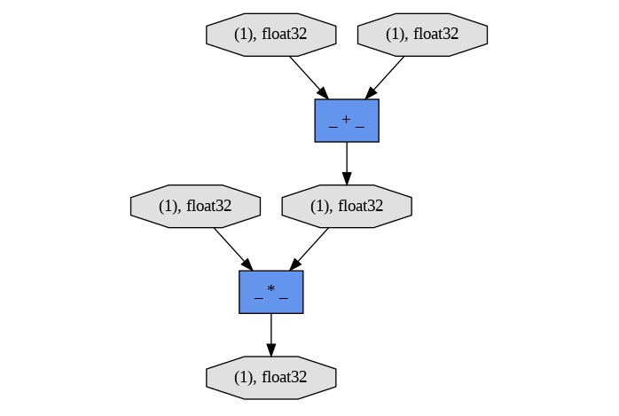
Note: It is recommended to use the Google colaboratory for better results.

Chainer - Dynamic vs Static Graphs

Dynamic Graphs

Dynamic graphs are also known as Define-by-Run graphs, which are a core feature of Chainer that distinguish it from other deep learning frameworks. Unlike static graphs which are predefined before any computation where as dynamic graphs are built on-the-fly as the computation occurs. This approach provides several advantages especially when dealing with complex models that require flexibility and adaptability.

Key Features of Dynamic Graphs in Chainer

Below are the key features of Dynamic Graphs in Chainer −

• Real-Time Graph Construction: In Chainer the computational graphs are built dynamically during the execution of the program. This real-time construction allows the graph to adapt immediately to the operations performed by making it easier to work with models that require flexibility.
• Flexibility in Model Design: The dynamic nature of Chainer's computational graphs supports the creation of models with variable structures such as those involving loops, conditionals or varying input sizes. This flexibility is particularly advantageous for tasks such as sequence processing and advanced neural network architectures.
• Efficient Memory Management: Chainer's approach to graph building allows it to manage memory more efficiently as the graph only exists as long as it is needed. Once an operation is completed the resources associated with it can be freed by reducing the overall memory footprint.
• Seamless Integration of Control Flow: Chainer's define-by-run model allows for the easy incorporation of control flow elements such as if-else statements and loops directly within the network. This integration supports complex models that require dynamic decision-making and branching logic.
• Immediate Feedback for Debugging: Since the graph is built during runtime, so any issues or errors in the network are immediately visible which simplifes the debugging process. This immediate feedback loop is beneficial for experimenting with different model architectures and quickly iterating on designs.
• Support for Complex and Custom Operations: Chainer's dynamic graphs can handle custom and complex operations by allowing for the creation of highly specialized network components. This capability is essential for research and applications that push the boundaries of standard neural network designs.
• Simplified Gradient Computation: During the backward pass the Chainer uses the dynamically generated graph to compute gradients efficiently. This ensures accurate and timely updates to model parameters, even when the network's structure changes during training.
• Ease of Prototyping and Experimentation: Chainer's dynamic graph system is ideal for prototyping new ideas as it allows for rapid testing and adjustment of different model configurations without the need to predefine the entire network structure.

Benefits of Dynamic graphics

Dynamic computational graphs in Chainer offer several practical benefits that enhance the flexibility, efficiency and speed of model development and experimentation. Let's see them in detail −

• Research Flexibility: Chainer is particularly well-suited for researchers and developers who need the freedom to experiment with different network architectures or make adjustments to existing models. The dynamic graph feature allows for easy modifications by enabling innovative approaches and rapid testing of new ideas.
• Handling Variable-Length Sequences: Chainer's dynamic graphs are especially useful in applications such as natural language processing or time-series forecasting where input sequences may vary in length. The ability to adjust the model on-the-fly to accommodate these variations without extensive reconfiguration is a significant advantage.
• Rapid Prototyping: The define-by-run approach of Chainer supports quick prototyping and iterative development. Developers can modify the model structure as needed without the hassle of re-compiling or predefining the entire computational graph by streamlining the development process and allowing for faster experimentation.

Example

Following is an example demonstrating the concept of dynamic graphs in Chainer where the computational graph is constructed dynamically based on the input or some other condition. This flexibility is particularly useful for models that involve decision-making during execution such as choosing different layers or operations based on runtime data −

import chainer
import chainer.functions as F
from chainer import Variable
from chainer.computational_graph import build_computational_graph
import numpy as np
from IPython.display import Image

# Define a function that uses dynamic control flow
def dynamic_graph_example(x, apply_relu):
   # Dynamic control flow: If apply_relu is True, use ReLU; otherwise, use Sigmoid
   if apply_relu:
      h = F.relu(x)
   else:
      h = F.sigmoid(x)
   
   # Another dynamic decision: apply a different operation
   if x.array.mean() > 0:
      y = F.sum(h)
   else:
      y = F.prod(h)
   
   return y

# Create a Variable (input) with random values
x = Variable(np.random.randn(5).astype(np.float32))

# Example 1: Apply ReLU and check the dynamic behavior
apply_relu = True
result_1 = dynamic_graph_example(x, apply_relu)

# Build the computational graph for the first result
g1 = build_computational_graph([result_1])

# Save the graph to a file
with open('dynamic_graph_relu.dot', 'w') as f:
   f.write(g1.dump())
print("Graph with ReLU has been saved as dynamic_graph_relu.dot")

# To convert .dot to .png using graphviz (in terminal or command prompt):
!dot -Tpng dynamic_graph_relu.dot -o dynamic_graph_relu.png
Image('dynamic_graph_relu.png')

Below is the output of displaying the dynamic graph in Chainer framework −

Graph with ReLU has been saved as dynamic_graph_relu.dot

Static Graphs

In Chainer the default behavior is to construct computational graphs dynamically. This means that the graph is built on-the-fly during the forward pass by allowing for flexibility in defining and executing the model. However a static graph refers to a graph that is predefined and fixed before the execution of any computations.

Although Chainer does not natively support static graphs as a primary feature we can still achieve a static-like behavior in Chainer by avoiding dynamic control flow and conditional operations.

Characteristics of Static Graphs

In a static graph approach the structure of the computational graph is predefined and unchanging throughout the execution of the model. This approach is contrast to dynamic graphs where the graph can adapt based on the data and computations performed. Here are the key characteristics of static graphs −

• Predefined Structure: The computational graph is fully defined before any data is processed. The arrangement of operations and data flow is established in advance and remains fixed.
• Fixed Architecture: The network's architecture includes all layers and their connections are specified beforehand. This architecture does not alter based on the input or intermediate results during runtime.
• No Dynamic Behavior: Static graphs do not include control flow constructs such as loops or conditionals that could modify the graph's structure during execution. All operations are predetermined and fixed.
• Consistent Execution: Every execution of the model follows the same graph structure which can simplify do optimization and debugging. The consistency in execution is due to the unchanging nature of the graph.
• Predefined Execution Plan: The plan for executing the computations is established before any actual data processing begins. This allows for optimization and efficient execution as the execution path is known in advance.

Mimicking Static Graphs in Chainer

Although Chainer's strength lies in its dynamic graph construction we can design our model in such a way that it mimics a static graph by adhering to the following principles −

• Avoid Conditional Operations: Ensure that the model does not include any conditionals or control flow that changes the network structure based on input data or intermediate computations.
• Predefine All Operations: All layers and operations should be defined at the beginning of the model. The flow of data through these operations should be fixed and not dependent on runtime conditions.

Advantages of Static Graphs

• Optimized Performance: Since the graph structure is fixed so the optimization techniques such as graph pruning, fusion of operations and efficient memory allocation can be applied more effectively.
• Predictable Execution: The absence of dynamic control flow ensures that the execution path is consistent which simplifies debugging and profiling as the model behavior is predictable.
• Enhanced Debugging: With a fixed structure it is easier to trace and diagnose issues in the computation which leads to more straightforward debugging and error tracking.
• Easier Model Sharing: A static graph can be more easily shared and reused across different platforms and environments, as the computation graph does not change based on input or runtime conditions.
• Efficient Resource Utilization: Static graphs allow for precompiled optimizations and resource allocations which potentially improves the runtime efficiency and reduce computational overhead.

Example

Below is the example which generates the Static computational graph in Chainer −

import chainer
import chainer.functions as F
import chainer.links as L
from chainer import Variable, Chain
from chainer.computational_graph import build_computational_graph
import numpy as np
from IPython.display import Image

# Define a model with a fixed architecture
class StaticGraphModel(Chain):
   def __init__(self):
      super(StaticGraphModel, self).__init__()
      with self.init_scope():
         self.l1 = L.Linear(None, 5)  # Input to hidden layer with 5 units
         self.l2 = L.Linear(5, 2)    # Hidden layer to output with 2 units

   def forward(self, x):
      h = F.relu(self.l1(x))  # Apply ReLU activation
      y = self.l2(h)        # Linear transformation to output
      return y

# Instantiate the model
model = StaticGraphModel()

# Create input variables
x = Variable(np.random.rand(3, 4).astype(np.float32))  # Batch of 3, 4 features each

# Forward pass (builds the computational graph)
y = model.forward(x)

# Build the computational graph
g = build_computational_graph([y])

# Save the graph to a file
with open('static_graph.dot', 'w') as f:
   f.write(g.dump())

print("Static graph has been saved as static_graph.dot")

# To convert .dot to .png using graphviz (in terminal or command prompt):
!dot -Tpng static_graph.dot -o static_graph.png
Image("static_graph.png")

The static graph created in chainer is displayed as follows −

Static graph has been saved as static_graph.dot

Dynamic Graph vs Static Graph

Following are the differences between Dynamic Graph and Static Graph −

Aspect	Dynamic Graphs	Static Graphs
Definition	Built on-the-fly during each forward pass.	Defined once before execution and reused thereafter.
Flexibility	Highly flexible, allowing varying structures per pass.	Less flexible, requiring a fixed structure.
Example Frameworks	Chainer, PyTorch	TensorFlow (pre-2.0), Theano
Advantages	Easy to debug using standard tools. Adaptable to complex, variable-length tasks. Code is intuitive and closely matches operations.	High performance due to extensive optimization. Easier to deploy in production environments. Advanced optimization opportunities.
Disadvantages	Potentially slower due to per-pass graph construction. Fewer compiler-level optimization opportunities.	Inflexibility in handling dynamic tasks. More challenging to debug.
Use Cases	Research, NLP, sequence-to-sequence tasks.	Production, tasks with consistent model structure.
Execution	Graph structure can change during each execution.	Same graph structure used for all executions.
Optimization	Limited optimization due to dynamic nature.	Extensive optimization possible for improved performance.

Chainer - Forward & Backward Propagation

Forward Propagation in Chainer

Forward propagation in Chainer refers to the process of passing input data through the layers of a neural network to compute the output. As we know Chainer is being a flexible deep learning framework, it allows dynamic computation graphs which means the graph is built on-the-fly as the data moves forward through the network.

During forward propagation each layer of the network applies a set of operations such as matrix multiplication, activation functions, etc. to the input data which progressively transforming it until the final output is produced. This output could be a prediction in tasks such as classification or regression.

In Chainer the forward propagation is typically handled by calling the model with the input data as an argument and the computation graph is constructed dynamically as this happens.

Steps involved in Forward Propagation

Forward propagation is a fundamental process in neural networks where input data is passed through the network layers to produce an output. The process involves applying a series of mathematical operations, typically involving matrix multiplications and activation functions to transform the input into the desired output. Here are the detailed steps involved in Forwad propagation −

• Input Layer: The process starts by feeding raw data into the network. Each input feature is assigned a weight that influences how it affects the next layers.
• Weighted Sum (Linear Transformation): For each layer the network computes a weighted sum of the inputs which is calculated as

  z = W . x + b
  

  where z is the weighted sum, W is the weight matrix, x is the input vector and b is the bias vector.

• Activation Function: The weighted sum z is passed through an activation function to introduce non-linearity into the model. Common functions such as ReLU (Rectified Linear Unit), Sigmoid and Tanh. For example, if we are using ReLU then the applying activation function will be as follows −

  a = ReLU(z)
  

  where a is result which is the transformed output of the activation function.

• Propagation Through Layers: The output from each layer serves as the input for the next layer. This process is iteratively applied across all hidden layers progressively refining the data representation.
• Output Layer: The final layer produces the network's prediction. The choice of activation function here depends on the task as mentioned below −
  • Classification: Softmax is used to generate class probabilities.
  • Regression: A linear function is used to output continuous values.
• Final Output: The output from the network is used to make predictions or decisions. During training this output is compared to the actual target values to compute the error which is used to update the weights through backpropagation.

Example

Here's an example of forward propagation in Chainer using a simple neural network. This network consists of an input layer, one hidden layer and an output layer. The below code shows how to perform forward propagation and obtain the network's output −

import chainer
import chainer.functions as F
import chainer.links as L
import numpy as np
from chainer import Variable

# Define the neural network model
class SimpleNN(chainer.Chain):
   def __init__(self):
      super(SimpleNN, self).__init__()
      with self.init_scope():
         self.l1 = L.Linear(3, 5)  # Input layer to hidden layer
         self.l2 = L.Linear(5, 2)  # Hidden layer to output layer

   def forward(self, x):
      # Compute the hidden layer output
      h = self.l1(x)
      print("Hidden layer (before activation):", h.data)
      
      # Apply ReLU activation function
      h = F.relu(h)
      print("Hidden layer (after ReLU):", h.data)
      
      # Compute the output layer
      y = self.l2(h)
      print("Output layer (before activation):", y.data)
      
      return y

# Create the model instance
model = SimpleNN()

# Prepare the input data
x = Variable(np.array([[1, 2, 3]], dtype=np.float32))  # Single sample with 3 features

# Perform forward propagation
output = model.forward(x)

# Display the final output
print("Final Output:", output.data)

Following is the output of the Forward Propagation −

Hidden layer (before activation): [[-3.2060928  -0.2460978   2.527906   -0.91410434  0.11754721]]
Hidden layer (after ReLU): [[0.       0.       2.527906   0.       0.11754721]]
Output layer (before activation): [[ 1.6746329  -0.21084023]]
Final Output: [[ 1.6746329  -0.21084023]]

Backward Propagation in Chainer

Backward propagation is a method used to compute the gradients of the loss function with respect to the parameters of a neural network. This process is essential for training the network by adjusting the weights to reduce the loss.

Steps in Backward Propagation

The Backward Propagation process consists of several key steps and each step is crucial for refining the model's parameters and enhancing its performance. Let's see them one by one in detail −

• Forward Pass: Input data is fed through the network by producing predictions. These predictions are then compared to the true targets using a loss function to calculate the prediction error.
• Loss Calculation: The loss function measures the discrepancy between predicted values and actual targets by providing a scalar value that reflects the model's performance.
• Backward Pass: The gradients of the loss function with respect to each network parameter are computed using the chain rule. This involves propagating the gradients backward through the network from the output layer to the input layer.
• Parameter Update: The computed gradients are used to adjust the network's parameters such as weights and biases. This adjustment is typically performed by an optimizer such as SGD or Adam which updates the parameters to minimize the loss function.

Example

Following is the example which shows how backward propagation works by printing the loss function in Chainer Framework −

import chainer
import chainer.functions as F
import chainer.links as L
from chainer import Chain, optimizers
import numpy as np

# Define a simple neural network
class MLP(Chain):
   def __init__(self):
      super(MLP, self).__init__()
      with self.init_scope():
         self.l1 = L.Linear(2, 3)  # Input layer to hidden layer
         self.l2 = L.Linear(3, 1)  # Hidden layer to output layer

   def forward(self, x):
      h = F.relu(self.l1(x))  # Forward pass through hidden layer
      y = self.l2(h)  # Forward pass through output layer
      return y

# Create a model and an optimizer
model = MLP()
optimizer = optimizers.SGD()
optimizer.setup(model)

# Sample input and target data
x = chainer.Variable(np.array([[1.0, 2.0]], dtype=np.float32))
t = chainer.Variable(np.array([[1.0]], dtype=np.float32))

# Forward pass
y = model.forward(x)
loss = F.mean_squared_error(y, t)  # Compute loss

# Backward pass
model.cleargrads()  # Clear previous gradients
loss.backward()  # Compute gradients
optimizer.update()  # Update parameters using the optimizer

print("Loss:", loss.data)

Below is the example which prints the loss function output of backward propagation −

Loss: 1.0728482

Chainer - Training and Evaluation

Training and evaluation in Chainer follow a flexible and dynamic approach due to its define-by-run architecture by allowing us to construct neural networks and perform tasks such as training, evaluation and optimization interactively. Heres a detailed explanation of the typical workflow for training and evaluating a neural network model using Chainer.

Training Process

Training a neural network in Chainer involves several key steps such as defining the model, preparing data, setting up the optimizer and iterating through the data for forward and backward passes. The main goal is to minimize the loss function by adjusting the models parameters using gradient-based optimization.

Here are the detailed steps involved in training process of a Neural Network in Chainer Frame work −

• Define the Model: In Chainer a model is typically defined as a subclass of chainer i.e. Chain which contains the layers of the neural network. Each layer is created as a link for example L.Linear for fully connected layers.
• Set Up the Optimizer: Chainer provides several optimizers Such as Adam, SGD, RMSprop, etc. These optimizers adjust the models parameters based on the gradients calculated during backpropagation.
• Prepare the Data: The training data is usually stored as NumPy arrays or can be handled by Chainer's Dataset and Iterator classes for larger datasets.
• Forward Pass: The model processes the input data through its layers by producing predictions or outputs.
• Compute Loss: A loss function such as F.mean_squared_error for regression or F.sigmoid_cross_entropy for binary classification measures how far off the models predictions are from the true labels.
• Backward Pass(Backpropagation): Gradients are computed by backpropagating the loss through the network. This allows the optimizer to adjust the weights of the model to minimize the loss.
• Update Parameters: The optimizer updates the model's parameters using the calculated gradients.

Example

Here is an example of simple neural network which shows how the training process carried out in Chainer −

import chainer
import chainer.functions as F
import chainer.links as L
from chainer import Chain, optimizers, Variable
import numpy as np

# Define a simple neural network model
class SimpleNN(Chain):
   def __init__(self):
      super(SimpleNN, self).__init__()
      with self.init_scope():
         self.l1 = L.Linear(None, 10) # Input to hidden layer 1
         self.l2 = L.Linear(10, 10)   # Hidden layer 1 to hidden layer 2
         self.l3 = L.Linear(10, 1)    # Hidden layer 2 to output layer

   def forward(self, x):
      h1 = F.relu(self.l1(x))
      h2 = F.relu(self.l2(h1))
      y = F.sigmoid(self.l3(h2))  # Sigmoid activation for binary classification
      return y

# Instantiate the model
model = SimpleNN()

# Set up an optimizer (Adam optimizer)
optimizer = optimizers.Adam()
optimizer.setup(model)

# Example training data
X_train = np.random.rand(100, 5).astype(np.float32)  # 100 samples, 5 features
y_train = np.random.randint(0, 2, size=(100, 1)).astype(np.int32)  # 100 binary labels

# Hyperparameters
n_epochs = 10
batch_size = 10

# Training loop
for epoch in range(n_epochs):
   for i in range(0, len(X_train), batch_size):
      # Prepare the batch
      x_batch = Variable(X_train[i:i+batch_size])
      y_batch = Variable(y_train[i:i+batch_size])

      # Forward pass (prediction)
      y_pred = model.forward(x_batch)

      # Compute the loss
      loss = F.sigmoid_cross_entropy(y_pred, y_batch)

      # Backward pass (compute gradients)
      model.cleargrads()
      loss.backward()

      # Update the parameters using the optimizer
      optimizer.update()

   print(f'Epoch {epoch+1}, Loss: {loss.array}')

Here is the output of the training process performed on a simple neural network −

Epoch 1, Loss: 0.668229877948761
Epoch 2, Loss: 0.668271541595459
Epoch 3, Loss: 0.6681589484214783
Epoch 4, Loss: 0.6679733991622925
Epoch 5, Loss: 0.6679850816726685
Epoch 6, Loss: 0.668184220790863
Epoch 7, Loss: 0.6684589982032776
Epoch 8, Loss: 0.6686227917671204
Epoch 9, Loss: 0.6686645746231079
Epoch 10, Loss: 0.6687664985656738

Evaluation Process

The evaluation process in Chainer involves assessing the performance of a trained neural network model on unseen data, usually the validation or test dataset. The primary goal of evaluation is to measure how well the model generalizes to new data which means its ability to make accurate predictions for inputs it hasn't seen during training process.

Below are the steps typically the Evaluation process follows −

• Disable Gradient Calculation: During evaluation we dont need to compute gradients. So it is efficient to disable them using chainer.using_config('train', False) to prevent unnecessary computations.
• Forward Pass: Pass the test data through the model to get predictions.
• Compute Evaluation Metrics: Depending on the task the metrics such as accuracy, precision, recall for classification or mean squared error for regression can be computed. This can be done using functions such as F.accuracy, F.mean_squared_error etc.
• Compare Predictions with Ground Truth: Evaluate the difference between the model's predictions and the actual labels in the test set.

Example

Here we are performing the evaluation process for the data which we trained in the above training process −

import chainer
import chainer.functions as F
import chainer.links as L
from chainer import Chain, optimizers, Variable
import numpy as np

# Define a simple neural network model
class SimpleNN(Chain):
   def __init__(self):
      super(SimpleNN, self).__init__()
      with self.init_scope():
         self.l1 = L.Linear(None, 10)  # Input to hidden layer 1
         self.l2 = L.Linear(10, 10)   # Hidden layer 1 to hidden layer 2
         self.l3 = L.Linear(10, 1)    # Hidden layer 2 to output layer

   def forward(self, x):
      h1 = F.relu(self.l1(x))
      h2 = F.relu(self.l2(h1))
      y = F.sigmoid(self.l3(h2))  # Sigmoid activation for binary classification
      return y

# Instantiate the model
model = SimpleNN()

# Set up an optimizer (Adam optimizer)
optimizer = optimizers.Adam()
optimizer.setup(model)

# Example training data
X_train = np.random.rand(100, 5).astype(np.float32)  # 100 samples, 5 features
y_train = np.random.randint(0, 2, size=(100, 1)).astype(np.int32)  # 100 binary labels

# Hyperparameters
n_epochs = 10
batch_size = 10

# Training loop
for epoch in range(n_epochs):
   for i in range(0, len(X_train), batch_size):
      # Prepare the batch
      x_batch = Variable(X_train[i:i+batch_size])
      y_batch = Variable(y_train[i:i+batch_size])

      # Forward pass (prediction)
      y_pred = model.forward(x_batch)

      # Compute the loss
      loss = F.sigmoid_cross_entropy(y_pred, y_batch)

      # Backward pass (compute gradients)
      model.cleargrads()
      loss.backward()

      # Update the parameters using the optimizer
      optimizer.update()

# Example test data
X_test = np.random.rand(10, 5).astype(np.float32)  # 10 samples, 5 features
y_test = np.random.randint(0, 2, size=(10, 1)).astype(np.int32)  # 10 binary labels

# Switch to evaluation mode (no gradients)
with chainer.using_config('train', False):
   y_pred = model.forward(Variable(X_test))

# Calculate the accuracy
accuracy = F.binary_accuracy(y_pred, Variable(y_test))

print("Test Accuracy:", accuracy.array)

Following is the test accuracy of the Evaluation of the process performed on the trained data −

Test Accuracy: 0.3

Saving and Loading Models

Chainer provides an easy way to save and load models using chainer.serializers function. This allows us to save the trained models parameters to a file and reload them later for evaluation or further training.

By using the below code we can save and load the model which we created above using chainer −

# Save the model
chainer.serializers.save_npz('simple_nn.model', model)
# Load the model
chainer.serializers.load_npz('simple_nn.model', model)

Chainer - Advanced Features

Chainer offers several advanced features that enhance its flexibility, efficiency and scalability in deep learning. These include GPU Acceleration with CuPy which leverages NVIDIA GPUs for faster computation, Mixed Precision Training which uses both 16-bit and 32-bit floating-point numbers to optimize performance and memory usage and Distributed Training which enables scaling across multiple GPUs or machines to handle larger models and datasets.

Additionally Chainer provides robust Debugging and Profiling Tools by allowing for real-time inspection and performance optimization of neural networks. These features collectively contribute to Chainer's capability to tackle complex and large-scale machine learning tasks efficiently.

GPU Acceleration with CuPy

GPU Acceleration with CuPy is an essential aspect of deep learning and numerical computation that leverages the computational power of GPUs to speed up operations. CuPy is a GPU-accelerated library that offers a NumPy-like API for performing operations on NVIDIA GPUs using CUDA. It is particularly useful in deep learning frameworks like Chainer for efficiently handling large-scale data and computations.

Key Features of CuPy

• NumPy-Like API: CuPy provides an interface similar to NumPy by making it easy to transition from CPU-based computations to GPU-accelerated computations with minimal code changes.
• CUDA Backend: CuPy utilizes CUDA, NVIDIA's parallel computing platform to perform operations on the GPU. This allows for significant performance improvements in numerical operations compared to CPU-based computations.
• Array Operations: It supports a wide range of array operations by including element-wise operations, reductions and linear algebra operations all accelerated by the GPU.
• Integration with Deep Learning Frameworks: CuPy integrates seamlessly with deep learning frameworks such as Chainer by allowing for efficient training and evaluation of models using GPU acceleration.

Example

In Chainer we can use CuPy arrays in place of NumPy arrays and Chainer will automatically leverage GPU acceleration for computations.Here is the example which integrates the Chainer with CuPy −

import chainer
import chainer.functions as F
import chainer.links as L
from chainer import Chain, optimizers, Variable
import cupy as cp

class SimpleNN(Chain):
   def __init__(self):
      super(SimpleNN, self).__init__()
      with self.init_scope():
         self.l1 = L.Linear(None, 10)
         self.l2 = L.Linear(10, 10)
         self.l3 = L.Linear(10, 1)

   def forward(self, x):
      h1 = F.relu(self.l1(x))
      h2 = F.relu(self.l2(h1))
      y = F.sigmoid(self.l3(h2))
      return y

# Initialize model and optimizer
model = SimpleNN()
optimizer = optimizers.Adam()
optimizer.setup(model)

# Example data (using CuPy arrays)
X_train = cp.random.rand(100, 5).astype(cp.float32)
y_train = cp.random.randint(0, 2, size=(100, 1)).astype(cp.float32)

# Convert to Chainer Variables
x_batch = Variable(X_train)
y_batch = Variable(y_train)

# Forward pass
y_pred = model.forward(x_batch)

# Compute loss
loss = F.sigmoid_cross_entropy(y_pred, y_batch)

# Backward pass and update
model.cleargrads()
loss.backward()
optimizer.update()

Mixed Precision Training

Mixed Precision Training is a technique used to accelerate deep learning training and reduce memory consumption by using different numerical precisions typically float16 and float32 for various parts of the model and training process. 16-bit Floating Point (FP16) is used for most of the calculations to save memory and improve computational speed and 32-bit Floating Point (FP32) is used for critical operations where precision is crucial such as maintaining the model's weights and gradients.

Key components of Mixed Precision Training

• Scaling Losses: To avoid underflow issues during the training with FP16, losses are scaled up (multiplied) before backpropagation. This scaling helps maintain the gradient's magnitude within a range that FP16 can handle.
• Loss Scaling: Dynamic loss scaling adjusts the scaling factor based on the gradients magnitude to prevent gradient overflow or underflow.
• FP16 Arithmetic: Computations such as matrix multiplications are performed in FP16 where possible and then results are converted to FP32 for accumulation and updates.

Example

Here is the example which shows how to work with Mixed Precision Training in chainer −

import chainer
import chainer.functions as F
import chainer.links as L
from chainer import Chain, optimizers, Variable
import numpy as np
import cupy as cp

# Define the model
class SimpleNN(Chain):
   def __init__(self):
      super(SimpleNN, self).__init__()
      with self.init_scope():
         self.l1 = L.Linear(None, 10)  # Input to hidden layer
         self.l2 = L.Linear(10, 10)   # Hidden layer to hidden layer
         self.l3 = L.Linear(10, 1)    # Hidden layer to output layer

   def __call__(self, x):
      h1 = F.relu(self.l1(x))
      h2 = F.relu(self.l2(h1))
      y = F.sigmoid(self.l3(h2))
      return y

# Mixed Precision Training Function
def mixed_precision_training(model, optimizer, X_train, y_train, n_epochs=10, batch_size=10):
   # Convert inputs to float16
   X_train = cp.asarray(X_train, dtype=cp.float16)
   y_train = cp.asarray(y_train, dtype=cp.float16)
   
   scaler = 1.0  # Initial scaling factor for gradients

   for epoch in range(n_epochs):
      for i in range(0, len(X_train), batch_size):
         x_batch = Variable(X_train[i:i+batch_size])
         y_batch = Variable(y_train[i:i+batch_size])

         # Forward pass
         y_pred = model(x_batch)

         # Compute loss (convert y_batch to float32 for loss calculation)
         loss = F.sigmoid_cross_entropy(y_pred, y_batch.astype(cp.float32))

         # Backward pass and weight update
         model.cleargrads()
         loss.backward()
         # Adjust gradients using the scaler
         for param in model.params():
            param.grad *= scaler

         optimizer.update()
         
         # Optionally, adjust scaler based on gradient norms
         # Here you can implement dynamic loss scaling if needed

      print(f'Epoch {epoch+1}, Loss: {loss.array}')

# Instantiate model and optimizer
model = SimpleNN()
optimizer = optimizers.Adam()
optimizer.setup(model)

# Example data (features and labels)
X_train = np.random.rand(100, 5).astype(np.float32)  # 100 samples, 5 features
y_train = np.random.randint(0, 2, size=(100, 1)).astype(np.float32)  # 100 binary labels

# Perform mixed precision training
mixed_precision_training(model, optimizer, X_train, y_train)

# Test data
X_test = np.random.rand(10, 5).astype(np.float32)  # 10 samples, 5 features
X_test = cp.asarray(X_test, dtype=cp.float16)  # Convert test data to float16
y_test = model(Variable(X_test))
print("Predictions:", y_test.data)

# Save the model
chainer.serializers.save_npz('simple_nn.model', model)

# Load the model
chainer.serializers.load_npz('simple_nn.model', model)

Distributed training

Distributed training in Chainer allows us to scale your model training across multiple GPUs or even multiple machines. Chainer provides tools to facilitate distributed training by making it possible to leverage parallel computing resources to accelerate the training process.

Key components in Distributed Training

Below are the key components in Distributed Training chainer −

• Data Parallelism: The most common approach in distributed training where the dataset is split across multiple GPUs or machines and each instance computes gradients based on its subset of data. Gradients are then averaged and applied to the model parameters.
• Model Parallelism: Involves splitting a single model across multiple GPUs or machines. Each device handles a portion of the model's parameters and computations. This approach is less common than data parallelism and often used for very large models.

Example

Here is the example of using the Distributed Training in Chainer −

import chainer
import chainer.functions as F
import chainer.links as L
from chainer import Chain, optimizers, training
from chainer.training import extensions
from chainer.dataset import DatasetMixin
import numpy as np

# Define the model
class SimpleNN(Chain):
   def __init__(self):
      super(SimpleNN, self).__init__()
      with self.init_scope():
         self.l1 = L.Linear(None, 10)
         self.l2 = L.Linear(10, 10)
         self.l3 = L.Linear(10, 1)

   def __call__(self, x):
      h1 = F.relu(self.l1(x))
      h2 = F.relu(self.l2(h1))
      y = F.sigmoid(self.l3(h2))
      return y

# Create a custom dataset
class RandomDataset(DatasetMixin):
   def __init__(self, size=100):
      self.data = np.random.rand(size, 5).astype(np.float32)
      self.target = np.random.randint(0, 2, size=(size, 1)).astype(np.float32)

   def __len__(self):
      return len(self.data)

   def get_example(self, i):
      return self.data[i], self.target[i]

# Prepare the dataset and iterators
dataset = RandomDataset()
train_iter = chainer.iterators.SerialIterator(dataset, batch_size=10)

# Set up the model and optimizer
model = SimpleNN()
optimizer = optimizers.Adam()
optimizer.setup(model)

# Set up the updater and trainer
updater = training.StandardUpdater(train_iter, optimizer, device=0)  # Use GPU 0
trainer = training.Trainer(updater, (10, 'epoch'), out='result')

# Add extensions
trainer.extend(extensions.Evaluator(train_iter, model, device=0))
trainer.extend(extensions.LogReport())
trainer.extend(extensions.PrintReport(['epoch', 'main/loss', 'validation/main/loss']))
trainer.extend(extensions.ProgressBar())

# Run the training
trainer.run()

Debugging and Profiling Tools

Chainer offers a range of debugging and profiling tools to help developers monitor and optimize neural network training. These tools aid in identifying bottlenecks, diagnosing issues and ensuring correctness in the models training and evaluation. Below is a breakdown of the key tools available −

• Define-by-Run Debugging Chainers define-by-run architecture allows the use of standard Python debugging tools such as print Statements which print intermediate values during the forward pass to inspect variable states and Python Debugger (pdb) is used step through code interactively to debug and inspect variables.
• Gradient Checking Chainer provides built-in support for gradient checking using chainer.gradient_check. This tool ensures that the computed gradients match the numerically estimated gradients.
• Chainer Profiler: The Chainer profiler helps measure the execution time of forward and backward passes. It identifies which operations are slowing down training.
• CuPy Profiler: For GPU-accelerated models using CuPy, Chainer allows you to profile GPU operations and optimize their execution.
• Memory Usage Profiling: Track memory consumption during training using the chainer.reporter module to ensure efficient memory management especially in large models.
• Handling Numerical Instabilities: Tools such as chainer.utils.isfinite() detect NaN or Inf values in tensors and gradient clipping can prevent exploding gradients.

These features make it easy to debug and optimize neural networks in Chainer while ensuring performance and stability during model training.

Example

Here is an example demonstrating how to use Chainers debugging and profiling tools to monitor the training of a simple neural network −

import chainer
import chainer.functions as F
import chainer.links as L
from chainer import Variable, Chain, optimizers, training, report
import numpy as np
from chainer import reporter, profiler

# Define a simple neural network model
class SimpleNN(Chain):
   def __init__(self):
      super(SimpleNN, self).__init__()
      with self.init_scope():
         self.l1 = L.Linear(None, 10)  # Input layer to hidden layer
         self.l2 = L.Linear(10, 1)    # Hidden layer to output layer

   def forward(self, x):
      h1 = F.relu(self.l1(x))   # ReLU activation
      y = self.l2(h1)
      return y

# Create a simple dataset
X_train = np.random.rand(100, 5).astype(np.float32)  # 100 samples, 5 features
y_train = np.random.rand(100, 1).astype(np.float32)  # 100 target values

# Instantiate the model and optimizer
model = SimpleNN()
optimizer = optimizers.Adam()
optimizer.setup(model)

# Enable the profiler
with profiler.profile() as prof:  # Start profiling
   for epoch in range(10):  # Training for 10 epochs
      for i in range(0, len(X_train), 10):  # Batch size of 10
         x_batch = Variable(X_train[i:i+10])
         y_batch = Variable(y_train[i:i+10])

         # Forward pass
         y_pred = model.forward(x_batch)
         
         # Debugging using print statements
         print(f'Epoch {epoch+1}, Batch {i//10+1}: Predicted {y_pred.data}, Actual {y_batch.data}')
         
         # Compute loss
         loss = F.mean_squared_error(y_pred, y_batch)
         
         # Clear gradients, backward pass, and update
         model.cleargrads()
         loss.backward()
         optimizer.update()

         # Report memory usage (for large models)
         reporter.report({'loss': loss})
         
   # Output profiling result
   prof.print()  # Print profiling information

# Check for NaN or Inf in weights
for param in model.params():
   assert chainer.utils.isfinite(param.array), "NaN or Inf found in parameters!"

print("Training complete!")

Chainer - Integration With Other Frameworks

Chainer can be integrated with various other deep learning and machine learning frameworks, libraries and tools to enhance its capabilities. These integrations allow developers to combine the flexibility and power of Chainers define-by-run architecture with the advantages of other systems.

In this tutorial we will discuss different common ways to integrate chainer with other frameworks −

Integration with NumPy and CuPy

Chainer's Integration with NumPy and CuPy enables smooth transitions between CPU and GPU computations by optimizing the efficiency of neural network training. NumPy is a core library for CPU-based numerical calculations while CuPy is its GPU equivalent which is designed for accelerated performance using CUDA.

NumPy Integration (CPU-Based Operations)

Chainer fully supports NumPy arrays by making it simple to use these arrays for computations on the CPU. We can easily pass NumPy arrays to Chainer's models and perform various deep learning tasks such as forward propagation, backward propagation and more. Chainer will treat these arrays as tensors and seamlessly execute operations.

Following is the example in which chainer operates directly on NumPy arrays for CPU-based calculations by showcasing how NumPy arrays can be incorporated easily −

import numpy as np
import chainer
from chainer import Variable

# Create a NumPy array
x_cpu = np.array([[1.0, 2.0], [3.0, 4.0]], dtype=np.float32)

# Convert NumPy array to a Chainer variable
x_var = Variable(x_cpu)

# Perform an operation using Chainer (CPU-based)
y_var = x_var + 2  # Add 2 to every element

print("Result (NumPy):", y_var.data)

Here is the outout of integrating the NumPy with Chainer −

Result (NumPy): [[3. 4.]
 [5. 6.]]

CuPy Integration (GPU-Based Operations)

Chainer provides seamless GPU acceleration through its integration with CuPy which is a library that mimics the NumPy API but runs on CUDA-enabled GPUs.

This means that we can switch between CPU and GPU simply by converting NumPy arrays to CuPy arrays and vice versa. Following is the example which integrates CuPy with the Chainer −

import cupy as cp
import chainer
from chainer import Variable

# Create a CuPy array (GPU-based)
x_gpu = cp.array([[1.0, 2.0], [3.0, 4.0]], dtype=cp.float32)

# Create a Chainer Variable from the CuPy array
x_var_gpu = Variable(x_gpu)

# Perform operations using Chainer (GPU-based)
y_var_gpu = x_var_gpu * 2  # Element-wise multiplication

print("Output (CuPy):", y_var_gpu.data)

Switching Between NumPy and CuPy

Chainer allows easy switching between NumPy and CuPy which is especially useful when we want to move data between CPU and GPU.

import numpy as np
import cupy as cp
import chainer
from chainer import Variable

# Create a NumPy array and move it to GPU
x_cpu = np.array([1.0, 2.0, 3.0], dtype=np.float32)
x_var = Variable(x_cpu)
x_var.to_gpu()  # Move the Variable to GPU

# Perform a computation on the GPU
y_var = x_var * 2

# Move the result back to CPU
y_var.to_cpu()

print("Output after moving back to CPU:", y_var.data)

Exporting Models to ONNX

ONNX is abbreviated as Open Neural Network Exchange which is an open-source format designed to facilitate integrating between various deep learning frameworks.

This is developed by Microsoft and Facebook which allows models to be trained in one framework and deployed in another by bridging gaps between tools such as PyTorch, TensorFlow, Chainer and more.

ONNX defines a standard set of operators and model representations that can be universally understood by making it easier for developers to share and deploy models across different platforms and hardware environments.

Steps for Exporting a Chainer Model to ONNX

Following are the steps to be used for exporting a chainer model to ONNX −

• Install ONNX Chainer Exporter: To export models from Chainer to ONNX format, we need to install the onnx-chainer package with the help of below code −

  pip install onnx-chainer
  

• Define a Chainer Model: First we need to create or load a trained Chainer model.
• Export the Model to ONNX Format: With the help of onnx_chainer.export function we can export the model.

Example

Here is the example of the model saved as simple_model.onnx which can be used in other frameworks or for deployment in ONNX-compatible environments.

import chainer
import chainer.links as L
import chainer.functions as F
from chainer import Chain, Variable
import numpy as np
import onnx_chainer

# Define a simple Chainer model
class SimpleModel(Chain):
    def __init__(self):
        super(SimpleModel, self).__init__()
        with self.init_scope():
            self.l1 = L.Linear(None, 3)  # Input to hidden layer

    def forward(self, x):
        return F.relu(self.l1(x))

# Instantiate the model
model = SimpleModel()

# Create dummy input data
x = np.random.rand(1, 5).astype(np.float32)

# Convert to Chainer variable
x_var = Variable(x)

# Forward pass
y = model.forward(x_var)

# Export the model to ONNX format
onnx_chainer.export(model, x, filename="simple_model.onnx")