Chainer - Computational Graphs

---

---

Computational graphs are crucial in deep learning for representing and executing the operations within neural networks. Chainer introduces a distinctive define-by-run approach which sets it apart by offering a dynamic and adaptable way to build and manage these graphs.

What is Computational Graph?

A Computational graph is a directed graph that represents the sequence of operations and dependencies involved in computing a function or performing a computation. Each node in the graph corresponds to a computational operation such as addition, multiplication or a more complex function while the edges represent the flow of data or the dependencies between these operations.

Chainer's Define-by-Run Approach

Chainer's Define-by-Run approach is a notable feature that distinguishes it from other deep learning frameworks. It enables the flexible and on-the-fly construction of computational graphs which streamlines the process of designing and testing complex neural network architectures.

Chainer's Define-by-Run approach enhances the flexibility, readability and efficiency of developing neural network models, making it easier to experiment with and refine complex architectures.

Following are the Key Features of the Define-by-Run Approach −

• Dynamic Graph Building: In Define-by-Run approach the computational graph is created dynamically during the execution of operations. Instead of predefining the entire graph structure it is assembled in real-time as the network processes data by accommodating variations in input and model structure.
• Model Design Flexibility: This approach allows for dynamic changes in model architecture. Developers can use control flow mechanisms like loops and conditionals within the network definition which makes it easier to design models that adapt to different conditions or inputs.
• Simplified Debugging:Debugging is more straightforward with Define-by-Run because code execution and graph construction occur simultaneously. Standard Python debugging tools such as print statements and interactive debugging which can be used without additional complexity.
• Adaptable to Complex Models: Define-by-Run is particularly advantageous for complex networks where the structure may vary based on the data or intermediate results. This adaptability is beneficial for tasks such as sequence-to-sequence learning or handling variable-length inputs.
• Readable and Intuitive Code: This approach promotes writing code that closely aligns with the mathematical operations being performed. This results in clearer and more understandable code as it mirrors the logic of the operations without the need for a static graph setup.

How Computational Graphs works in Chainer?

AS we all know Chainer's computational graph operates using its Define-by-Run approach which allows for dynamic and flexible model construction. Following we can see how Chainer's computational graphs work −

• Dynamic Construction: Unlike static graph frameworks where the entire graph must be defined before execution, Chainer constructs the computational graph dynamically. As operations are executed the Chainer builds the graph in real-time. This allows for immediate adjustments and modifications based on the operations performed.
• Forward Pass: During the forward pass the Chainer processes the input data through the network. As each operation is carried out then the Chainer creates nodes and edges in the computational graph to represent the operations and data flow. This means that the graph structure evolves as computations occur.
• Backward Pass: Once the forward pass is complete and the output is obtained then Chainer uses the dynamically constructed graph to compute gradients during the backward pass. The gradients are calculated through automatic differentiation where the chain rule is applied to the graph to update the model parameters.
• Flexible Model Design: Chainer's approach allows for the inclusion of conditional statements, loops and other control flow mechanisms within the network definition. This flexibility is particularly useful for complex models that require dynamic architecture adjustments based on input data or intermediate results
• Execution and Debugging: The Define-by-Run model means that debugging and code execution happen concurrently. Developers can use standard Python debugging tools like print statements and interactive debuggers to inspect and understand the behavior of the model, as the computational graph is being built and executed.
• Adaptability: Chainer's dynamic graph construction is ideal for tasks involving variable-length inputs or sequences. The graph can adapt in real-time to the changing structure of the input data by making it suitable for applications such as sequence-to-sequence models or variable-length sequences.

Advantages of Computational Graph

Chainer's computational graphs offer several advantages that make it a powerful tool for developing neural networks −

• Dynamic Graph Construction: Chainer builds computational graphs dynamically during runtime rather than requiring a static definition upfront. This allows for greater flexibility in model design as the graph can adapt based on input data and intermediate computations.
• Flexibility in Model Design: The dynamic nature of Chainer's computational graphs supports complex architectures that involve varying structures such as those with conditional operations or loops. This is particularly useful for models like recurrent neural networks (RNNs) and sequence-to-sequence models.
• Ease of Debugging: Since the graph is constructed during execution the developers can easily debug the model using standard Python debugging tools. This means that errors can be traced and fixed more intuitively without needing to delve into a pre-built static graph.
• Adaptive to Variable-Length Inputs: Chainer's approach is well-suited for handling variable-length inputs, such as sequences of text or time series data. The graph adapts dynamically to the length and structure of the input by making it ideal for tasks like natural language processing.
• Simplified Code Structure: The define-by-run approach allows for more natural and readable code as it closely follows the logic of the operations being performed. Developers can write models in a way that mirrors the mathematical operations without having to map them to a pre-defined graph structure.
• Support for Control Flow Operations: Chainer's computational graphs can include control flow operations such as loops and conditionals directly within the network architecture. This is a significant advantage for models that require complex decision-making processes or iterative computations.
• Real-Time Graph Modifications: The ability to modify the graph in real-time during execution allows for experimenting with different architectures and making adjustments on the fly without the need to redefine the entire model.

Applications of Computational Graph

Computational graphs are essential in many fields due to their ability to visually and mathematically represent complex computations. Here are some key applications of computational graphs −

• Deep Learning: Computational graphs model the flow of data through neural networks by enabling efficient forward and backward propagation for training deep learning models.
• Optimization: They are used to visualize and compute gradients in optimization problems by helping to find the best parameters for a given objective function.
• Automatic Differentiation: Computational graphs enable automatic differentiation, is a technique used to compute derivatives efficiently which is crucial for training machine learning models.
• Probabilistic Modeling: In probabilistic graphical models the computational graphs represent dependencies between random variables by facilitating inference and learning in complex models like Bayesian networks.
• Compilers and Execution Engines: Computational graphs are employed in modern compilers and execution engines such as TensorFlow and PyTorch to optimize and execute operations efficiently on different hardware architectures.
• Signal Processing: The Computational Graphs are used to design and analyze signal processing algorithms by providing a structured way to represent and optimize signal transformations and filtering operations.

Example

To display a computational graph in Chainer we can use the chainer.computational_graph module to create a visual representation of the graph. Here are the steps how to display the computational graph in chainer framework −

• Install Chainer and Graphviz: Ensure we have Chainer and Graphviz installed in our working environment, if not we can install them using pip with the help of below code −

pip install chainer
pip install graphviz

Create a Simple Computational Graph: In this we will create a simple computational graph that computes the function z=(x+y)w and displays it.

Convert the .dot File to an Image: The computational graph output will be saved as a .dot file which can be converted to an image using Graphviz. To perform this we have to run the following code −

dot -Tpng graph.dot -o graph.png

This will generate a graph.png file that visually represents the computational graph.

Now here is the example that demonstrates how to build a simple computational graph and display it using Chainer −

import chainer
import chainer.functions as F
import chainer.links as L
from chainer import Variable, Chain
from chainer.computational_graph import build_computational_graph
import numpy as np

# Define a simple model as a Chain
class SimpleModel(Chain):
   def __init__(self):
      super(SimpleModel, self).__init__()
      with self.init_scope():
         self.l1 = L.Linear(None, 1)  # A linear layer

   def forward(self, x, y, w):
      # Perform addition and multiplication
      h = x + y
      z = h * w
      return z

# Instantiate the model
model = SimpleModel()

# Create input variables using numpy arrays
x = Variable(np.random.normal(size=(1,)).astype(np.float32))
y = Variable(np.random.normal(size=(1,)).astype(np.float32))
w = Variable(np.random.normal(size=(1,)).astype(np.float32))

# Forward pass
z = model.forward(x, y, w)

# Build the computational graph
g = build_computational_graph([z])

# Save the graph to a file
with open('graph.dot', 'w') as f:
   f.write(g.dump())

print("Graph has been saved as graph.dot")
# converting the .dot file to png
!dot -Tpng graph.dot -o graph.png

from IPython.display import Image
Image('graph.png')

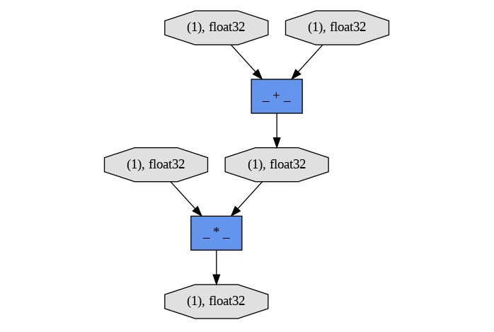
Following is the output of the computational graph created for the function z=(x+y)w −

Graph has been saved as graph.dot

Note: It is recommended to use the Google colaboratory for better results.