Caffe2 Tutorial
Caffe2 - Home
Caffe2 - Introduction
Caffe2 - Overview
Caffe2 - Installation
Verifying Access to Pre-Trained Models
Image Classification Using Pre-Trained Model
Caffe2 - Creating Your Own Network
Caffe2 - Defining Complex Networks
Caffe2 Useful Resources
Caffe2 - Quick Guide
Caffe2 - Useful Resources
Caffe2 - Discussion

Caffe2 - Quick Guide

Caffe2 - Introduction

Last couple of years, Deep Learning has become a big trend in Machine Learning. It has been successfully applied to solve previously unsolvable problems in Vision, Speech Recognition and Natural Language Processing (NLP). There are many more domains in which Deep Learning is being applied and has shown its usefulness.

Caffe (Convolutional Architecture for Fast Feature Embedding) is a deep learning framework developed at Berkeley Vision and Learning Center (BVLC). The Caffe project was created by Yangqing Jia during his Ph.D. at University of California - Berkeley. Caffe provides an easy way to experiment with deep learning. It is written in C++ and provides bindings for Python and Matlab.

It supports many different types of deep learning architectures such as CNN (Convolutional Neural Network), LSTM (Long Short Term Memory) and FC (Fully Connected). It supports GPU and is thus, ideally suited for production environments involving deep neural networks. It also supports CPU-based kernel libraries such as NVIDIA, CUDA Deep Neural Network library (cuDNN) and Intel Math Kernel Library (Intel MKL).

In April 2017, U.S. based social networking service company Facebook announced Caffe2, which now includes RNN (Recurrent Neural Networks) and in March 2018, Caffe2 was merged into PyTorch. Caffe2 creators and community members have created models for solving various problems. These models are available to the public as pre-trained models. Caffe2 helps the creators in using these models and creating one’s own network for making predictions on the dataset.

Before we go into the details of Caffe2, let us understand the difference between machine learning and deep learning. This is necessary to understand how models are created and used in Caffe2.

Machine Learning v/s Deep Learning

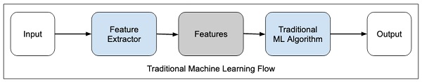
In any machine learning algorithm, be it a traditional one or a deep learning one, the selection of features in the dataset plays an extremely important role in getting the desired prediction accuracy. In traditional machine learning techniques, the feature selection is done mostly by human inspection, judgement and deep domain knowledge. Sometimes, you may seek help from a few tested algorithms for feature selection.

The traditional machine learning flow is depicted in the figure below −

In deep learning, the feature selection is automatic and is a part of deep learning algorithm itself. This is shown in the figure below −

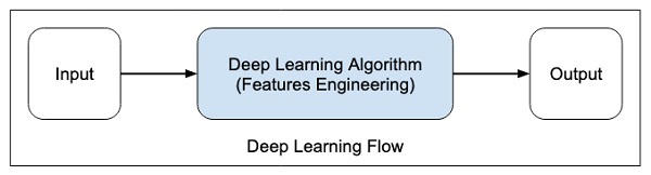
In deep learning algorithms, feature engineering is done automatically. Generally, feature engineering is time-consuming and requires a good expertise in domain. To implement the automatic feature extraction, the deep learning algorithms typically ask for huge amount of data, so if you have only thousands and tens of thousands of data points, the deep learning technique may fail to give you satisfactory results.

With larger data, the deep learning algorithms produce better results compared to traditional ML algorithms with an added advantage of less or no feature engineering.

Caffe2 - Overview

Now, as you have got some insights into deep learning, let us get an overview of what is Caffe.

Training a CNN

Let us learn the process for training a CNN for classifying images. The process consists of the following steps −

Data Preparation − In this step, we center-crop the images and resize them so that all images for training and testing would be of the same size. This is usually done by running a small Python script on the image data.
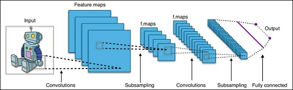
Model Definition − In this step, we define a CNN architecture. The configuration is stored in .pb (protobuf) file. A typical CNN architecture is shown in figure below.
Solver Definition − We define the solver configuration file. Solver does the model optimization.
Model Training − We use the built-in Caffe utility to train the model. The training may take a considerable amount of time and CPU usage. After the training is completed, Caffe stores the model in a file, which can later on be used on test data and final deployment for predictions.

What’s New in Caffe2

In Caffe2, you would find many ready-to-use pre-trained models and also leverage the community contributions of new models and algorithms quite frequently. The models that you create can scale up easily using the GPU power in the cloud and also can be brought down to the use of masses on mobile with its cross-platform libraries.

The improvements made in Caffe2 over Caffe may be summarized as follows −

Mobile deployment
New hardware support
Support for large-scale distributed training
Quantized computation
Stress tested on Facebook

Pretrained Model Demo

The Berkeley Vision and Learning Center (BVLC) site provides demos of their pre- trained networks. One such network for image classification is available on the link stated herewith https://caffe2.ai/docs/learn-more#null__caffe-neural-network-for-image-classification and is depicted in the screenshot below.

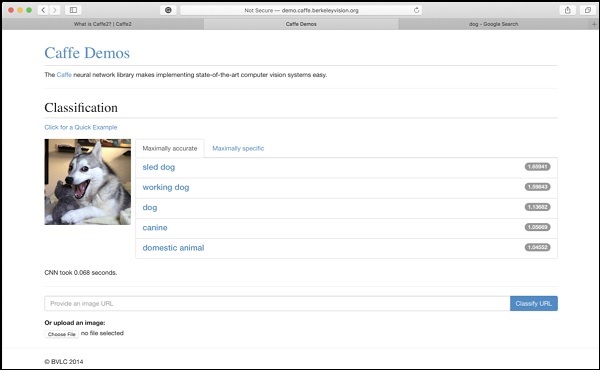
In the screenshot, the image of a dog is classified and labelled with its prediction accuracy. It also says that it took just 0.068 seconds to classify the image. You may try an image of your own choice by specifying the image URL or uploading the image itself in the options given at the bottom of the screen.

Caffe2 - Installation

Now, that you have got enough insights on the capabilities of Caffe2, it is time to experiment Caffe2 on your own. To use the pre-trained models or to develop your models in your own Python code, you must first install Caffe2 on your machine.

On the installation page of Caffe2 site which is available at the link https://caffe2.ai/docs/getting-started.html you would see the following to select your platform and install type.

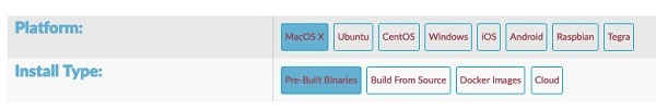
As you can see in the above screenshot, Caffe2 supports several popular platforms including the mobile ones.

Now, we shall understand the steps for MacOS installation on which all the projects in this tutorial are tested.

MacOS Installation

The installation can be of four types as given below −

Pre-Built Binaries
Build From Source
Docker Images
Cloud

Depending upon your preference, select any of the above as your installation type. The instructions given here are as per the Caffe2 installation site for pre-built binaries. It uses Anaconda for Jupyter environment. Execute the following command on your console prompt

pip install torch_nightly -f 
https://download.pytorch.org/whl/nightly/cpu/torch_nightly.html

In addition to the above, you will need a few third-party libraries, which are installed using the following commands −

conda install -c anaconda setuptools
conda install -c conda-forge graphviz  
conda install -c conda-forge hypothesis
conda install -c conda-forge ipython
conda install -c conda-forge jupyter
conda install -c conda-forge matplotlib
conda install -c anaconda notebook
conda install -c anaconda pydot
conda install -c conda-forge python-nvd3
conda install -c anaconda pyyaml
conda install -c anaconda requests
conda install -c anaconda scikit-image
conda install -c anaconda scipy

Some of the tutorials in the Caffe2 website also require the installation of zeromq, which is installed using the following command −

conda install -c anaconda zeromq

Windows/Linux Installation

Execute the following command on your console prompt −

conda install -c pytorch pytorch-nightly-cpu

As you must have noticed, you would need Anaconda to use the above installation. You will need to install the additional packages as specified in the MacOS installation.

Testing Installation

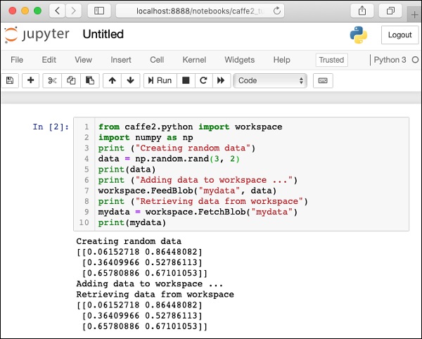
To test your installation, a small Python script is given below, which you can cut and paste in your Juypter project and execute.

from caffe2.python import workspace
import numpy as np
print ("Creating random data")
data = np.random.rand(3, 2)
print(data)
print ("Adding data to workspace ...")
workspace.FeedBlob("mydata", data)
print ("Retrieving data from workspace")
mydata = workspace.FetchBlob("mydata")
print(mydata)

When you execute the above code, you should see the following output −

Creating random data
[[0.06152718 0.86448082]
[0.36409966 0.52786113]
[0.65780886 0.67101053]]
Adding data to workspace ...
Retrieving data from workspace
[[0.06152718 0.86448082]
[0.36409966 0.52786113]
[0.65780886 0.67101053]]

The screenshot of the installation test page is shown here for your quick reference −

Now, that you have installed Caffe2 on your machine, proceed to install the tutorial applications.

Tutorial Installation

Download the tutorials source using the following command on your console −

git clone --recursive https://github.com/caffe2/tutorials caffe2_tutorials

After the download is completed, you will find several Python projects in the caffe2_tutorials folder in your installation directory. The screenshot of this folder is given for your quick perusal.

/Users/yourusername/caffe2_tutorials

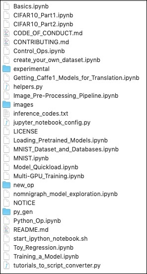
You can open some of these tutorials to see what the Caffe2 code looks like. The next two projects described in this tutorial are largely based on the samples shown above.

It is now time to do some Python coding of our own. Let us understand, how to use a pre-trained model from Caffe2. Later, you will learn to create your own trivial neural network for training on your own dataset.

Caffe2 - Verifying Access to Pre-Trained Models

Before you learn to use a pre-trained model in your Python application, let us first verify that the models are installed on your machine and are accessible through the Python code.

When you install Caffe2, the pre-trained models are copied in the installation folder. On the machine with Anaconda installation, these models are available in the following folder.

anaconda3/lib/python3.7/site-packages/caffe2/python/models

Check out the installation folder on your machine for the presence of these models. You can try loading these models from the installation folder with the following short Python script −

CAFFE_MODELS = os.path.expanduser("/anaconda3/lib/python3.7/site-packages/caffe2/python/models")
INIT_NET = os.path.join(CAFFE_MODELS, 'squeezenet', 'init_net.pb')
PREDICT_NET = os.path.join(CAFFE_MODELS, 'squeezenet', 'predict_net.pb')
print(INIT_NET)
print(PREDICT_NET)

When the script runs successfully, you will see the following output −

/anaconda3/lib/python3.7/site-packages/caffe2/python/models/squeezenet/init_net.pb
/anaconda3/lib/python3.7/site-packages/caffe2/python/models/squeezenet/predict_net.pb

This confirms that the squeezenet module is installed on your machine and is accessible to your code.

Now, you are ready to write your own Python code for image classification using Caffe2 squeezenet pre-trained module.

Image Classification Using Pre-Trained Model

In this lesson, you will learn to use a pre-trained model to detect objects in a given image. You will use squeezenet pre-trained module that detects and classifies the objects in a given image with a great accuracy.

Open a new Juypter notebook and follow the steps to develop this image classification application.

Importing Libraries

First, we import the required packages using the below code −

from caffe2.proto import caffe2_pb2
from caffe2.python import core, workspace, models
import numpy as np
import skimage.io
import skimage.transform
from matplotlib import pyplot
import os
import urllib.request as urllib2
import operator

Next, we set up a few variables −

INPUT_IMAGE_SIZE = 227
mean = 128

The images used for training will obviously be of varied sizes. All these images must be converted into a fixed size for accurate training. Likewise, the test images and the image which you want to predict in the production environment must also be converted to the size, the same as the one used during training. Thus, we create a variable above called INPUT_IMAGE_SIZE having value 227. Hence, we will convert all our images to the size 227x227 before using it in our classifier.

We also declare a variable called mean having value 128, which is used later for improving the classification results.

Next, we will develop two functions for processing the image.

Image Processing

The image processing consists of two steps. First one is to resize the image, and the second one is to centrally crop the image. For these two steps, we will write two functions for resizing and cropping.

Image Resizing

First, we will write a function for resizing the image. As said earlier, we will resize the image to 227x227. So let us define the function resize as follows −

def resize(img, input_height, input_width):

We obtain the aspect ratio of the image by dividing the width by the height.

original_aspect = img.shape[1]/float(img.shape[0])

If the aspect ratio is greater than 1, it indicates that the image is wide, that to say it is in the landscape mode. We now adjust the image height and return the resized image using the following code −

if(original_aspect>1):
   new_height = int(original_aspect * input_height)
   return skimage.transform.resize(img, (input_width,
   new_height), mode='constant', anti_aliasing=True, anti_aliasing_sigma=None)

If the aspect ratio is less than 1, it indicates the portrait mode. We now adjust the width using the following code −

if(original_aspect<1):
   new_width = int(input_width/original_aspect)
   return skimage.transform.resize(img, (new_width,
   input_height), mode='constant', anti_aliasing=True, anti_aliasing_sigma=None)

If the aspect ratio equals 1, we do not make any height/width adjustments.

if(original_aspect == 1):
   return skimage.transform.resize(img, (input_width,
   input_height), mode='constant', anti_aliasing=True, anti_aliasing_sigma=None)

The full function code is given below for your quick reference −

def resize(img, input_height, input_width):
   original_aspect = img.shape[1]/float(img.shape[0])
   if(original_aspect>1):
      new_height = int(original_aspect * input_height)
      return skimage.transform.resize(img, (input_width,
	   new_height), mode='constant', anti_aliasing=True, anti_aliasing_sigma=None)
   if(original_aspect<1):
         new_width = int(input_width/original_aspect)
         return skimage.transform.resize(img, (new_width,
         input_height), mode='constant', anti_aliasing=True, anti_aliasing_sigma=None)
   if(original_aspect == 1):
         return skimage.transform.resize(img, (input_width,
         input_height), mode='constant', anti_aliasing=True, anti_aliasing_sigma=None)

We will now write a function for cropping the image around its center.

Image Cropping

We declare the crop_image function as follows −

def crop_image(img,cropx,cropy):

We extract the dimensions of the image using the following statement −

y,x,c = img.shape

We create a new starting point for the image using the following two lines of code −

startx = x//2-(cropx//2)
starty = y//2-(cropy//2)

Finally, we return the cropped image by creating an image object with the new dimensions −

return img[starty:starty+cropy,startx:startx+cropx]

The entire function code is given below for your quick reference −

def crop_image(img,cropx,cropy):
   y,x,c = img.shape
   startx = x//2-(cropx//2)
   starty = y//2-(cropy//2)
   return img[starty:starty+cropy,startx:startx+cropx]

Now, we will write code to test these functions.

Processing Image

Firstly, copy an image file into images subfolder within your project directory. tree.jpg file is copied in the project. The following Python code loads the image and displays it on the console −

img = skimage.img_as_float(skimage.io.imread("images/tree.jpg")).astype(np.float32)
print("Original Image Shape: " , img.shape)
pyplot.figure()
pyplot.imshow(img)
pyplot.title('Original image')

The output is as follows −

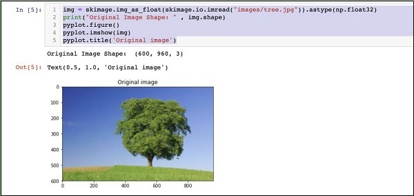
Note that size of the original image is 600 x 960. We need to resize this to our specification of 227 x 227. Calling our earlier-defined resizefunction does this job.

img = resize(img, INPUT_IMAGE_SIZE, INPUT_IMAGE_SIZE)
print("Image Shape after resizing: " , img.shape)
pyplot.figure()
pyplot.imshow(img)
pyplot.title('Resized image')

The output is as given below −

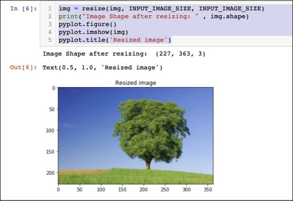
Note that now the image size is 227 x 363. We need to crop this to 227 x 227 for the final feed to our algorithm. We call the previously-defined crop function for this purpose.

img = crop_image(img, INPUT_IMAGE_SIZE, INPUT_IMAGE_SIZE)
print("Image Shape after cropping: " , img.shape)
pyplot.figure()
pyplot.imshow(img)
pyplot.title('Center Cropped')

Below mentioned is the output of the code −

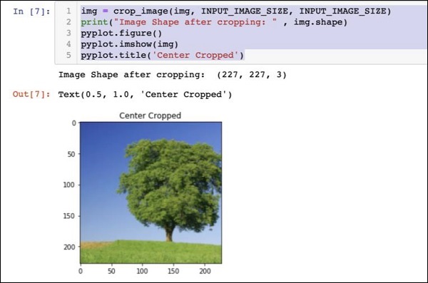
At this point, the image is of size 227 x 227 and is ready for further processing. We now swap the image axes to extract the three colours into three different zones.

img = img.swapaxes(1, 2).swapaxes(0, 1)
print("CHW Image Shape: " , img.shape)

Given below is the output −

CHW Image Shape: (3, 227, 227)

Note that the last axis has now become the first dimension in the array. We will now plot the three channels using the following code −

pyplot.figure()
for i in range(3):
   pyplot.subplot(1, 3, i+1)
   pyplot.imshow(img[i])
   pyplot.axis('off')
   pyplot.title('RGB channel %d' % (i+1))

The output is stated below −

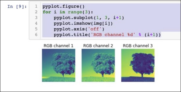
Finally, we do some additional processing on the image such as converting Red Green Blue to Blue Green Red (RGB to BGR), removing mean for better results and adding batch size axis using the following three lines of code −

# convert RGB --> BGR
img = img[(2, 1, 0), :, :]
# remove mean
img = img * 255 - mean
# add batch size axis
img = img[np.newaxis, :, :, :].astype(np.float32)

At this point, your image is in NCHW format and is ready for feeding into our network. Next, we will load our pre-trained model files and feed the above image into it for prediction.

Predicting Objects in Processed Image

We first setup the paths for the init and predict networks defined in the pre-trained models of Caffe.

Setting Model File Paths

Remember from our earlier discussion, all the pre-trained models are installed in the models folder. We set up the path to this folder as follows −

CAFFE_MODELS = os.path.expanduser("/anaconda3/lib/python3.7/site-packages/caffe2/python/models")

We set up the path to the init_net protobuf file of the squeezenet model as follows −

INIT_NET = os.path.join(CAFFE_MODELS, 'squeezenet', 'init_net.pb')

Likewise, we set up the path to the predict_net protobuf as follows −

PREDICT_NET = os.path.join(CAFFE_MODELS, 'squeezenet', 'predict_net.pb')

We print the two paths for diagnosis purpose −

print(INIT_NET)
print(PREDICT_NET)

The above code along with the output is given here for your quick reference −

CAFFE_MODELS = os.path.expanduser("/anaconda3/lib/python3.7/site-packages/caffe2/python/models")
INIT_NET = os.path.join(CAFFE_MODELS, 'squeezenet', 'init_net.pb')
PREDICT_NET = os.path.join(CAFFE_MODELS, 'squeezenet', 'predict_net.pb')
print(INIT_NET)
print(PREDICT_NET)

The output is mentioned below −

/anaconda3/lib/python3.7/site-packages/caffe2/python/models/squeezenet/init_net.pb
/anaconda3/lib/python3.7/site-packages/caffe2/python/models/squeezenet/predict_net.pb

Next, we will create a predictor.

Creating Predictor

We read the model files using the following two statements −

with open(INIT_NET, "rb") as f:
   init_net = f.read()
with open(PREDICT_NET, "rb") as f:
   predict_net = f.read()

The predictor is created by passing pointers to the two files as parameters to the Predictor function.

p = workspace.Predictor(init_net, predict_net)

The p object is the predictor, which is used for predicting the objects in any given image. Note that each input image must be in NCHW format as what we have done earlier to our tree.jpg file.

Predicting Objects

To predict the objects in a given image is trivial - just executing a single line of command. We call run method on the predictor object for an object detection in a given image.

results = p.run({'data': img})

The prediction results are now available in the results object, which we convert to an array for our readability.

results = np.asarray(results)

Print the dimensions of the array for your understanding using the following statement −

print("results shape: ", results.shape)

The output is as shown below −

results shape: (1, 1, 1000, 1, 1)

We will now remove the unnecessary axis −

preds = np.squeeze(results)

The topmost predication can now be retrieved by taking the max value in the preds array.

curr_pred, curr_conf = max(enumerate(preds), key=operator.itemgetter(1))
print("Prediction: ", curr_pred)
print("Confidence: ", curr_conf)

The output is as follows −

Prediction: 984
Confidence: 0.89235985

As you see the model has predicted an object with an index value 984 with 89% confidence. The index of 984 does not make much sense to us in understanding what kind of object is detected. We need to get the stringified name for the object using its index value. The kind of objects that the model recognizes along with their corresponding index values are available on a github repository.

Now, we will see how to retrieve the name for our object having index value of 984.

Stringifying Result

We create a URL object to the github repository as follows −

codes = "https://gist.githubusercontent.com/aaronmarkham/cd3a6b6ac0
71eca6f7b4a6e40e6038aa/raw/9edb4038a37da6b5a44c3b5bc52e448ff09bfe5b/alexnet_codes"

We read the contents of the URL −

response = urllib2.urlopen(codes)

The response will contain a list of all codes and its descriptions. Few lines of the response are shown below for your understanding of what it contains −

5: 'electric ray, crampfish, numbfish, torpedo',
6: 'stingray',
7: 'cock',
8: 'hen',
9: 'ostrich, Struthio camelus',
10: 'brambling, Fringilla montifringilla',

We now iterate the entire array to locate our desired code of 984 using a for loop as follows −

for line in response:
   mystring = line.decode('ascii')
   code, result = mystring.partition(":")[::2]
   code = code.strip()
   result = result.replace("'", "")
   if (code == str(curr_pred)):
      name = result.split(",")[0][1:]
      print("Model predicts", name, "with", curr_conf, "confidence")

When you run the code, you will see the following output −

Model predicts rapeseed with 0.89235985 confidence

You may now try the model on another image.

Predicting a Different Image

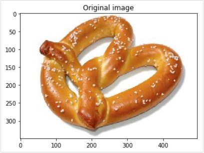
To predict another image, simply copy the image file into the images folder of your project directory. This is the directory in which our earlier tree.jpg file is stored. Change the name of the image file in the code. Only one change is required as shown below

img = skimage.img_as_float(skimage.io.imread("images/pretzel.jpg")).astype(np.float32)

The original picture and the prediction result are shown below −

The output is mentioned below −

Model predicts pretzel with 0.99999976 confidence

As you see the pre-trained model is able to detect objects in a given image with a great amount of accuracy.

Full Source

The full source for the above code that uses a pre-trained model for object detection in a given image is mentioned here for your quick reference −

def crop_image(img,cropx,cropy):
   y,x,c = img.shape
   startx = x//2-(cropx//2)
   starty = y//2-(cropy//2)
   return img[starty:starty+cropy,startx:startx+cropx]
img = skimage.img_as_float(skimage.io.imread("images/pretzel.jpg")).astype(np.float32)
print("Original Image Shape: " , img.shape)
pyplot.figure()
pyplot.imshow(img)
pyplot.title('Original image')
img = resize(img, INPUT_IMAGE_SIZE, INPUT_IMAGE_SIZE)
print("Image Shape after resizing: " , img.shape)
pyplot.figure()
pyplot.imshow(img)
pyplot.title('Resized image')
img = crop_image(img, INPUT_IMAGE_SIZE, INPUT_IMAGE_SIZE)
print("Image Shape after cropping: " , img.shape)
pyplot.figure()
pyplot.imshow(img)
pyplot.title('Center Cropped')
img = img.swapaxes(1, 2).swapaxes(0, 1)
print("CHW Image Shape: " , img.shape)
pyplot.figure()
for i in range(3):
pyplot.subplot(1, 3, i+1)
pyplot.imshow(img[i])
pyplot.axis('off')
pyplot.title('RGB channel %d' % (i+1))
# convert RGB --> BGR
img = img[(2, 1, 0), :, :]
# remove mean
img = img * 255 - mean
# add batch size axis
img = img[np.newaxis, :, :, :].astype(np.float32)
CAFFE_MODELS = os.path.expanduser("/anaconda3/lib/python3.7/site-packages/caffe2/python/models")
INIT_NET = os.path.join(CAFFE_MODELS, 'squeezenet', 'init_net.pb')
PREDICT_NET = os.path.join(CAFFE_MODELS, 'squeezenet', 'predict_net.pb')
print(INIT_NET)
print(PREDICT_NET)
with open(INIT_NET, "rb") as f:
   init_net = f.read()
with open(PREDICT_NET, "rb") as f:
   predict_net = f.read()
p = workspace.Predictor(init_net, predict_net)
results = p.run({'data': img})
results = np.asarray(results)
print("results shape: ", results.shape)
preds = np.squeeze(results)
curr_pred, curr_conf = max(enumerate(preds), key=operator.itemgetter(1))
print("Prediction: ", curr_pred)
print("Confidence: ", curr_conf)
codes = "https://gist.githubusercontent.com/aaronmarkham/cd3a6b6ac071eca6f7b4a6e40e6038aa/raw/9edb4038a37da6b5a44c3b5bc52e448ff09bfe5b/alexnet_codes"
response = urllib2.urlopen(codes)
for line in response:
   mystring = line.decode('ascii')
   code, result = mystring.partition(":")[::2]
   code = code.strip()
   result = result.replace("'", "")
   if (code == str(curr_pred)):
      name = result.split(",")[0][1:]
      print("Model predicts", name, "with", curr_conf, "confidence")

By this time, you know how to use a pre-trained model for doing the predictions on your dataset.

What’s next is to learn how to define your neural network (NN) architectures in Caffe2 and train them on your dataset. We will now learn how to create a trivial single layer NN.

Caffe2 - Creating Your Own Network

In this lesson, you will learn to define a single layer neural network (NN) in Caffe2 and run it on a randomly generated dataset. We will write code to graphically depict the network architecture, print input, output, weights, and bias values. To understand this lesson, you must be familiar with neural network architectures, its terms and mathematics used in them.

Network Architecture

Let us consider that we want to build a single layer NN as shown in the figure below −

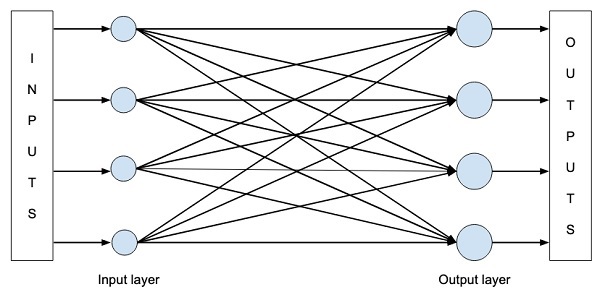
Mathematically, this network is represented by the following Python code −

Y = X * W^T + b

Where X, W, b are tensors and Y is the output. We will fill all three tensors with some random data, run the network and examine the Y output. To define the network and tensors, Caffe2 provides several Operator functions.

Caffe2 Operators

In Caffe2, Operator is the basic unit of computation. The Caffe2 Operator is represented as follows.

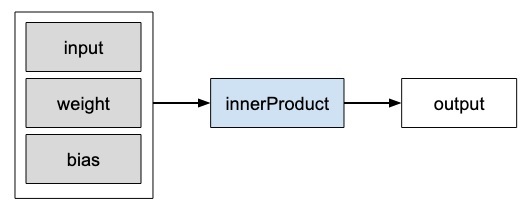
Caffe2 provides an exhaustive list of operators. For the network that we are designing currently, we will use the operator called FC, which computes the result of passing an input vector X into a fully connected network with a two-dimensional weight matrix W and a single-dimensional bias vector b. In other words, it computes the following mathematical equation

Y = X * W^T + b

Where X has dimensions (M x k), W has dimensions (n x k) and b is (1 x n). The output Y will be of dimension (M x n), where M is the batch size.

For the vectors X and W, we will use the GaussianFill operator to create some random data. For generating bias values b, we will use ConstantFill operator.

We will now proceed to define our network.

Creating Network

First of all, import the required packages −

from caffe2.python import core, workspace

Next, define the network by calling core.Net as follows −

net = core.Net("SingleLayerFC")

The name of the network is specified as SingleLayerFC. At this point, the network object called net is created. It does not contain any layers so far.

Creating Tensors

We will now create the three vectors required by our network. First, we will create X tensor by calling GaussianFill operator as follows −

X = net.GaussianFill([], ["X"], mean=0.0, std=1.0, shape=[2, 3], run_once=0)

The X vector has dimensions 2 x 3 with the mean data value of 0,0 and standard deviation of 1.0.

Likewise, we create W tensor as follows −

W = net.GaussianFill([], ["W"], mean=0.0, std=1.0, shape=[5, 3], run_once=0)

The W vector is of size 5 x 3.

Finally, we create bias b matrix of size 5.

b = net.ConstantFill([], ["b"], shape=[5,], value=1.0, run_once=0)

Now, comes the most important part of the code and that is defining the network itself.

Defining Network

We define the network in the following Python statement −

Y = X.FC([W, b], ["Y"])

We call FC operator on the input data X. The weights are specified in W and bias in b. The output is Y. Alternatively, you may create the network using the following Python statement, which is more verbose.

Y = net.FC([X, W, b], ["Y"])

At this point, the network is simply created. Until we run the network at least once, it will not contain any data. Before running the network, we will examine its architecture.

Printing Network Architecture

Caffe2 defines the network architecture in a JSON file, which can be examined by calling the Proto method on the created net object.

print (net.Proto())

This produces the following output −

name: "SingleLayerFC"
op {
   output: "X"
   name: ""
   type: "GaussianFill"
   arg {
      name: "mean"
      f: 0.0
   }
   arg {
      name: "std"
      f: 1.0
   }
   arg {
      name: "shape"
      ints: 2
      ints: 3
   }
   arg {
      name: "run_once"
      i: 0
   }
}
op {
   output: "W"
   name: ""
   type: "GaussianFill"
   arg {
      name: "mean"
      f: 0.0
   }
   arg {
      name: "std"
      f: 1.0
   }
   arg {
      name: "shape"
      ints: 5
      ints: 3
   }
   arg {
      name: "run_once"
      i: 0
   }
}
op {
   output: "b"
   name: ""
   type: "ConstantFill"
   arg {
      name: "shape"
      ints: 5
   }
   arg {
      name: "value"
      f: 1.0
   }
   arg {
      name: "run_once"
      i: 0
   }
}
op {
   input: "X"
   input: "W"
   input: "b"
   output: "Y"
   name: ""
   type: "FC"
}

As you can see in the above listing, it first defines the operators X, W and b. Let us examine the definition of W as an example. The type of W is specified as GausianFill. The mean is defined as float 0.0, the standard deviation is defined as float 1.0, and the shape is 5 x 3.

op {
   output: "W"
   name: "" type: "GaussianFill"
   arg {
      name: "mean" 
	   f: 0.0
   }
   arg { 
      name: "std" 
      f: 1.0
   }
   arg { 
      name: "shape" 
      ints: 5 
      ints: 3
   }
   ...
}

Examine the definitions of X and b for your own understanding. Finally, let us look at the definition of our single layer network, which is reproduced here

op {
   input: "X"
   input: "W"
   input: "b"
   output: "Y"
   name: ""
   type: "FC"
}

Here, the network type is FC (Fully Connected) with X, W, b as inputs and Y is the output. This network definition is too verbose and for large networks, it will become tedious to examine its contents. Fortunately, Caffe2 provides a graphical representation for the created networks.

Network Graphical Representation

To get the graphical representation of the network, run the following code snippet, which is essentially only two lines of Python code.

from caffe2.python import net_drawer
from IPython import display
graph = net_drawer.GetPydotGraph(net, rankdir="LR")
display.Image(graph.create_png(), width=800)

When you run the code, you will see the following output −

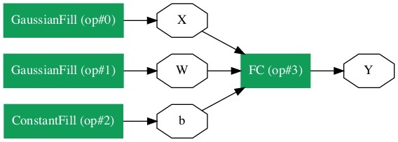
For large networks, the graphical representation becomes extremely useful in visualizing and debugging network definition errors.

Finally, it is now time to run the network.

Running Network

You run the network by calling the RunNetOnce method on the workspace object −

workspace.RunNetOnce(net)

After the network is run once, all our data that is generated at random would be created, fed into the network and the output will be created. The tensors which are created after running the network are called blobs in Caffe2. The workspace consists of the blobs you create and store in memory. This is quite similar to Matlab.

After running the network, you can examine the blobs that the workspace contains using the following print command

print("Blobs in the workspace: {}".format(workspace.Blobs()))

You will see the following output −

Blobs in the workspace: ['W', 'X', 'Y', 'b']

Note that the workspace consists of three input blobs − X, W and b. It also contains the output blob called Y. Let us now examine the contents of these blobs.

for name in workspace.Blobs():
   print("{}:\n{}".format(name, workspace.FetchBlob(name)))

You will see the following output −

W:
[[ 1.0426593 0.15479846 0.25635982]
[-2.2461145 1.4581774 0.16827184]
[-0.12009818 0.30771437 0.00791338]
[ 1.2274994 -0.903331 -0.68799865]
[ 0.30834186 -0.53060573 0.88776857]]
X:
[[ 1.6588869e+00 1.5279824e+00 1.1889904e+00]
[ 6.7048723e-01 -9.7490678e-04 2.5114202e-01]]
Y:
[[ 3.2709925 -0.297907 1.2803618 0.837985 1.7562964]
[ 1.7633215 -0.4651525 0.9211631 1.6511179 1.4302125]]
b:
[1. 1. 1. 1. 1.]

Note that the data on your machine or as a matter of fact on every run of the network would be different as all inputs are created at random. You have now successfully defined a network and run it on your computer.

Caffe2 - Defining Complex Networks

In the previous lesson, you learned to create a trivial network and learned how to execute it and examine its output. The process for creating complex networks is similar to the process described above. Caffe2 provides a huge set of operators for creating complex architectures. You are encouraged to examine the Caffe2 documentation for a list of operators. After studying the purpose of various operators, you would be in a position to create complex networks and train them. For training the network, Caffe2 provides several predefined computation units - that is the operators. You will need to select the appropriate operators for training your network for the kind of problem that you are trying to solve.

Once a network is trained to your satisfaction, you can store it in a model file similar to the pre-trained model files you used earlier. These trained models may be contributed to Caffe2 repository for the benefits of other users. Or you may simply put the trained model for your own private production use.

Summary

Caffe2, which is a deep learning framework allows you to experiment with several kinds of neural networks for predicting your data. Caffe2 site provides many pre-trained models. You learned to use one of the pre-trained models for classifying objects in a given image. You also learned to define a neural network architecture of your choice. Such custom networks can be trained using many predefined operators in Caffe. A trained model is stored in a file which can be taken into a production environment.