- Apache Bench - Home
- Apache Bench - Overview
- Apache Bench - Environment Setup
- Testing Our Sample Application
- Testing Multiple URLs Concurrently
- Preparation for Testing Dynamic Pages
- Sequential Test Cases for Dynamic Pages
- Comparison of Outputs
Apache Bench - Environment Setup
In this chapter, we will guide you how to set up your environment for Apache Bench on your VPS.
System Requirement
Memory − 128 MB
Disk Space − No minimum requirement
Operating System − No minimum requirement
Installing Apache Bench
Apache Bench is a stand-alone application, and has no dependencies on the Apache web server installation. The following is a two-step process to install Apache Bench.
Step 1 − Update package database.
# apt-get update
Please note that symbol # before a terminal command means that root user is issuing that command.
Step 2 − Install apache2 utils package to get access to Apache Bench.
# apt-get install apache2-utils
Apache Bench is now installed. If you want to test a web application hosted on the same VPS, then it is enough to install the Apache web server only −
# apt-get install apache2
Being an Apache utility, Apache Bench is automatically installed on installation of the Apache web server.
Verifying Apache Bench Installation
Let us now see how to verify Apache Bench Installation. The following code will help verify the installation −
# ab -V
Output
This is ApacheBench, Version 2.3 <$Revision: 1604373 $>
Copyright 1996 Adam Twiss, Zeus Technology Ltd, http://www.zeustech.net/
Licensed to The Apache Software Foundation, http://www.apache.org/
When you see the above terminal output, it means you have successfully installed Apache Bench.
Creating a Privileged Sudo User
From the safety point of view, it is considered a good practice for system administrator to create a sudo user instead of working as root. We will create a test user, named test, for the purpose −
# useradd -m -d /home/test -g sudo test
Let us set the password for the new user −
# passwd test
System will prompt for a new password for the user test. You can enter a simple password as we are just testing, and not deploying to the production server. Usually the sudo command will prompt you to provide the sudo user password; it is recommended not to use complicated password as the process becomes cumbersome.
Output
Enter new UNIX password:
Retype new UNIX password:
passwd: password updated successfully
Testing Apache.org Website
In this section, we will test the Apache.org Website. Let us first switch to the sudo user test −
# su test
To begin with, we will test the website of Apache organization, https://www.apache.org/. We will first run the command, and then understand the output −
$ ab -n 100 -c 10 https://www.apache.org/
Here -n is the number of requests to perform for the benchmarking session. The default is to just perform a single request which usually leads to non-representative benchmarking results.
And -c is the concurrency and denotes the number of multiple requests to perform at a time. Default is one request at a time.
So in this test, Apache Bench will make 100 requests with concurrency 10 to the Apache organization server.
Output
This is ApacheBench, Version 2.3 <$Revision: 1604373 $>
Copyright 1996 Adam Twiss, Zeus Technology Ltd, http://www.zeustech.net/
Licensed to The Apache Software Foundation, http://www.apache.org/

Benchmarking www.apache.org (be patient).....done

Server Software:        Apache/2.4.7
Server Hostname:        www.apache.org
Server Port:            443
SSL/TLS Protocol:       TLSv1.2,ECDHE-RSA-AES256-GCM-SHA384,2048,256

Document Path:          /
Document Length:        58769 bytes

Concurrency Level:      10
Time taken for tests:   1.004 seconds
Complete requests:      100
Failed requests:        0
Total transferred:      5911100 bytes
HTML transferred:       5876900 bytes
Requests per second:    99.56 [#/sec] (mean)
Time per request:       100.444 [ms] (mean)
Time per request:       10.044 [ms] (mean, across all concurrent requests)
Transfer rate:          5747.06 [Kbytes/sec] received

Connection Times (ms)
              min  mean[+/-sd] median   max
Connect:       39   46  30.9     41     263
Processing:    37   40  21.7     38     255
Waiting:       12   15  21.7     13     230
Total:         77   86  37.5     79     301

Percentage of the requests served within a certain time (ms)
  50%     79
  66%     79
  75%     80
  80%     80
  90%     82
  95%     84
  98%    296
  99%    301
 100%    301 (longest request)
Having run our first test, it will be easy to recognize the pattern of use for this command which is as follows −
# ab [options .....] URL
where,
ab − Apache Bench command
options − flags for particular task we want to perform
URL − path url we want to test
Understanding the Output Values
We need to understand the different metrics to understand the various output values returned by ab. Here goes the list −
Server Software − It is the name of the web server returned in the HTTP header of the first successful return.
Server Hostname − It is the DNS or IP address given on the command line.
Server Port − It is the port to which ab is connecting. If no port is given on the command line, this will default to 80 for http and 443 for https.
SSL/TLS Protocol − This is the protocol parameter negotiated between the client and server. This will only be printed if SSL is used.
Document Path − This is the request URI parsed from the command line string.
Document Length − It is the size in bytes of the first successfully returned document. If the document length changes during testing, the response is considered an error.
Concurrency Level − This is the number of concurrent clients (equivalent to web browsers) used during the test.
Time Taken for Tests − This is the time taken from the moment the first socket connection is created to the moment the last response is received.
Complete Requests − The number of successful responses received.
Failed Requests − The number of requests that were considered a failure. If the number is greater than zero, another line will be printed showing the number of requests that failed due to connecting, reading, incorrect content length, or exceptions.
Total Transferred − The total number of bytes received from the server. This number is essentially the number of bytes sent over the wire.
HTML Transferred − The total number of document bytes received from the server. This number excludes bytes received in HTTP headers
Requests per second − This is the number of requests per second. This value is the result of dividing the number of requests by the total time taken.
Time per request − The average time spent per request. The first value is calculated with the formula concurrency * timetaken * 1000 / done while the second value is calculated with the formula timetaken * 1000 / done
Transfer rate − The rate of transfer as calculated by the formula totalread / 1024 / timetaken.
Quick Analysis of the Load Testing Output
Having learned about the headings of the output values from the ab command, let us try to analyze and understand the output values for our initial test −
Apache organisation is using their own web Server Software − Apache (version 2.4.7)
Server is listening on Port 443 because of https. Had it been http, it would have been 80 (default).
Total data transferred is 58769 bytes for 100 requests.
Test completed in 1.004 seconds. There are no failed requests.
Requests per seconds − 99.56. This is considered a pretty good number.
Time per request − 100.444 ms (for 10 concurrent requests). So across all requests, it is 100.444 ms/10 = 10.044 ms.
Transfer rate − 1338.39 [Kbytes/sec] received.
In connection time statistics, you can observe that many requests had to wait for few seconds. This may be due to apache web server putting requests in wait queue.
In our first test, we had tested an application (i.e., www.apache.org) hosted on a different server. In the later part of the tutorial, we will be testing our sample web-applications hosted on the same server from which we will be running the ab tests. This is for the ease of learning and demonstration purpose. Ideally, the host node and testing node should be different for accurate measurement.
To better learn ab, you should compare and observe how the output values vary for different cases as we move forward in this tutorial.
Plotting the Output of Apache Bench
Here we will plot the relevant outcome to see how much time the server takes as the number of requests increases. For that, we will add the -g option in the previous command followed by the file name (here out.data) in which the ab output data will be saved −
$ ab -n 100 -c 10 -g out.data https://www.apache.org/
Let us now see the out.data before we create a plot −
$ less out.data
Output
starttime       seconds ctime   dtime   ttime   wait
Tue May 30 12:11:37 2017        1496160697      40      38      77      13
Tue May 30 12:11:37 2017        1496160697      42      38      79      13
Tue May 30 12:11:37 2017        1496160697      41      38      80      13
...
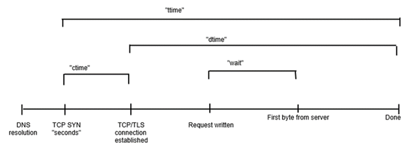
Let us now understand the column headers in the out.data file −
starttime − This is the date and time at which the call started.
seconds − Same as starttime but in the Unix timestamp format (date -d @1496160697 returns starttime output).
ctime − This is the Connection Time.
dtime − This is the Processing Time.
ttime − This is the Total Time (it is the sum of ctime and dtime, mathematically ttime = ctime + dtime).
wait − This is the Waiting Time.
For a pictorial visualization of how these multiple items are related to each other, take a look at the following image −
If we are working over terminal or where graphics are not available, gnuplot is a great option. We will quickly understand it by going through the following steps.
Let us install and launch gnuplot −
$ sudo apt-get install gnuplot
$ gnuplot
Output
G N U P L O T
Version 4.6 patchlevel 6    last modified September 2014
Build System: Linux x86_64

Copyright (C) 1986-1993, 1998, 2004, 2007-2014
Thomas Williams, Colin Kelley and many others

gnuplot home:     http://www.gnuplot.info
faq, bugs, etc:   type "help FAQ"
immediate help:   type "help"  (plot window: hit 'h')

Terminal type set to 'qt'
gnuplot>
As we are working over terminal and supposing that graphics are not available, we can choose the dumb terminal which will give output in ASCII over the terminal itself. This helps us get an idea what our plot looks like with this quick tool. Let us now prepare the terminal for ASCII plot.
gnuplot> set terminal dumb
Output
Terminal type set to 'dumb'
Options are 'feed  size 79, 24'
As, our gnuplot terminal is now ready for ASCII plot, let us plot the data from the out.data file −
gnuplot> plot "out.data" using 9 w l
Output
  1400 ++-----+------+-----+------+------+------+------+-----+------+-----++
       +      +      +     +      +      +      +"out.data" using 9 ****** +
       |                                                                   |
  1200 ++                       ********************************************
       |     *******************                                           |
  1000 ++    *                                                            ++
       |     *                                                             |
       |     *                                                             |
   800 ++   *                                                             ++
       |    *                                                              |
       |    *                                                              |
   600 ++   *                                                             ++
       |    *                                                              |
       |    *                                                              |
   400 ++   *                                                             ++
       |    *                                                              |
   200 ++   *                                                             ++
       |    *                                                              |
       +****  +      +     +      +      +      +      +     +      +      +
     0 ++-----+------+-----+------+------+------+------+-----+------+-----++
       0      10     20    30     40     50     60     70    80     90    100
We have plotted the ttime, total time (in ms) from column 9, with respect to the number of requests. We can notice that for the initial ten requests, the total time was in the nearly 100 ms, for next 30 requests (from 10th to 40th), it increased to 1100 ms, and so on. Your plot must be different depending on your out.data.
