- Scikit Image – Introduction
- Scikit Image - Image Processing
- Scikit Image - Numpy Images
- Scikit Image - Image datatypes
- Scikit Image - Using Plugins
- Scikit Image - Image Handlings
- Scikit Image - Reading Images
- Scikit Image - Writing Images
- Scikit Image - Displaying Images
- Scikit Image - Image Collections
- Scikit Image - Image Stack
- Scikit Image - Multi Image
- Scikit Image - Data Visualization
- Scikit Image - Using Matplotlib
- Scikit Image - Using Ploty
- Scikit Image - Using Mayavi
- Scikit Image - Using Napari
- Scikit Image - Color Manipulation
- Scikit Image - Alpha Channel
- Scikit Image - Conversion b/w Color & Gray Values
- Scikit Image - Conversion b/w RGB & HSV
- Scikit Image - Conversion to CIE-LAB Color Space
- Scikit Image - Conversion from CIE-LAB Color Space
- Scikit Image - Conversion to luv Color Space
- Scikit Image - Conversion from luv Color Space
- Scikit Image - Image Inversion
- Scikit Image - Painting Images with Labels
- Scikit Image - Contrast & Exposure
- Scikit Image - Contrast
- Scikit Image - Contrast enhancement
- Scikit Image - Exposure
- Scikit Image - Histogram Matching
- Scikit Image - Histogram Equalization
- Scikit Image - Local Histogram Equalization
- Scikit Image - Tinting gray-scale images
- Scikit Image - Image Transformation
- Scikit Image - Scaling an image
- Scikit Image - Rotating an Image
- Scikit Image - Warping an Image
- Scikit Image - Affine Transform
- Scikit Image - Piecewise Affine Transform
- Scikit Image - ProjectiveTransform
- Scikit Image - EuclideanTransform
- Scikit Image - Radon Transform
- Scikit Image - Line Hough Transform
- Scikit Image - Probabilistic Hough Transform
- Scikit Image - Circular Hough Transforms
- Scikit Image - Elliptical Hough Transforms
- Scikit Image - Polynomial Transform
- Scikit Image - Image Pyramids
- Scikit Image - Pyramid Gaussian Transform
- Scikit Image - Pyramid Laplacian Transform
- Scikit Image - Swirl Transform
- Scikit Image - Morphological Operations
- Scikit Image - Erosion
- Scikit Image - Dilation
- Scikit Image - Black & White Tophat Morphologies
- Scikit Image - Convex Hull
- Scikit Image - Generating footprints
- Scikit Image - Isotopic Dilation & Erosion
- Scikit Image - Isotopic Closing & Opening of an Image
- Scikit Image - Skelitonizing an Image
- Scikit Image - Morphological Thinning
- Scikit Image - Masking an image
- Scikit Image - Area Closing & Opening of an Image
- Scikit Image - Diameter Closing & Opening of an Image
- Scikit Image - Morphological reconstruction of an Image
- Scikit Image - Finding local Maxima
- Scikit Image - Finding local Minima
- Scikit Image - Removing Small Holes from an Image
- Scikit Image - Removing Small Objects from an Image
- Scikit Image - Filters
- Scikit Image - Image Filters
- Scikit Image - Median Filter
- Scikit Image - Mean Filters
- Scikit Image - Morphological gray-level Filters
- Scikit Image - Gabor Filter
- Scikit Image - Gaussian Filter
- Scikit Image - Butterworth Filter
- Scikit Image - Frangi Filter
- Scikit Image - Hessian Filter
- Scikit Image - Meijering Neuriteness Filter
- Scikit Image - Sato Filter
- Scikit Image - Sobel Filter
- Scikit Image - Farid Filter
- Scikit Image - Scharr Filter
- Scikit Image - Unsharp Mask Filter
- Scikit Image - Roberts Cross Operator
- Scikit Image - Lapalace Operator
- Scikit Image - Window Functions With Images
- Scikit Image - Thresholding
- Scikit Image - Applying Threshold
- Scikit Image - Otsu Thresholding
- Scikit Image - Local thresholding
- Scikit Image - Hysteresis Thresholding
- Scikit Image - Li thresholding
- Scikit Image - Multi-Otsu Thresholding
- Scikit Image - Niblack and Sauvola Thresholding
- Scikit Image - Restoring Images
- Scikit Image - Rolling-ball Algorithm
- Scikit Image - Denoising an Image
- Scikit Image - Wavelet Denoising
- Scikit Image - Non-local means denoising for preserving textures
- Scikit Image - Calibrating Denoisers Using J-Invariance
- Scikit Image - Total Variation Denoising
- Scikit Image - Shift-invariant wavelet denoising
- Scikit Image - Image Deconvolution
- Scikit Image - Richardson-Lucy Deconvolution
- Scikit Image - Recover the original from a wrapped phase image
- Scikit Image - Image Inpainting
- Scikit Image - Registering Images
- Scikit Image - Image Registration
- Scikit Image - Masked Normalized Cross-Correlation
- Scikit Image - Registration using optical flow
- Scikit Image - Assemble images with simple image stitching
- Scikit Image - Registration using Polar and Log-Polar
- Scikit Image - Feature Detection
- Scikit Image - Dense DAISY Feature Description
- Scikit Image - Histogram of Oriented Gradients
- Scikit Image - Template Matching
- Scikit Image - CENSURE Feature Detector
- Scikit Image - BRIEF Binary Descriptor
- Scikit Image - SIFT Feature Detector and Descriptor Extractor
- Scikit Image - GLCM Texture Features
- Scikit Image - Shape Index
- Scikit Image - Sliding Window Histogram
- Scikit Image - Finding Contour
- Scikit Image - Texture Classification Using Local Binary Pattern
- Scikit Image - Texture Classification Using Multi-Block Local Binary Pattern
- Scikit Image - Active Contour Model
- Scikit Image - Canny Edge Detection
- Scikit Image - Marching Cubes
- Scikit Image - Foerstner Corner Detection
- Scikit Image - Harris Corner Detection
- Scikit Image - Extracting FAST Corners
- Scikit Image - Shi-Tomasi Corner Detection
- Scikit Image - Haar Like Feature Detection
- Scikit Image - Haar Feature detection of coordinates
- Scikit Image - Hessian matrix
- Scikit Image - ORB feature Detection
- Scikit Image - Additional Concepts
- Scikit Image - Render text onto an image
- Scikit Image - Face detection using a cascade classifier
- Scikit Image - Face classification using Haar-like feature descriptor
- Scikit Image - Visual image comparison
- Scikit Image - Exploring Region Properties With Pandas
Texture Classification Using Local Binary Pattern
Local Binary Pattern (LBP) is a powerful texture descriptor used in image analysis. It involves comparing the pixel values of a central point with those of its neighboring pixels, resulting in a binary outcome. This tutorial explores how to perform texture classification using LBP.
LBP examines the points surrounding a central pixel and determines whether these surrounding points are greater or less than the central point, resulting in a binary representation.
The scikit image library offers the local_binary_pattern() function within its feature module to perform this task.
Using the skimage.feature.local_binary_pattern() function
The feature.local_binary_pattern() function is used to compute the Local Binary Pattern (LBP) of a 2D grayscale image. LBP is a visual descriptor often used in texture classification.
Syntax
Following is the syntax of this function −
skimage.feature.local_binary_pattern(image, P, R, method='default')
Parameters
The function accepts the following parameters −
image (M, N) array: This parameter is the input 2D grayscale image on which to compute the LBP.
P (int): It specifies the number of circularly symmetric neighbor set points. This quantizes the angular space.
R (float): This parameter defines the radius of the circle used for spatial resolution in the LBP operator.
method (str, optional): This parameter is used to determine the LBP pattern. The available options are −
default: This is the original local binary pattern. It is grayscale invariant but not rotation invariant.
ror: This is an extension of the default pattern and is both grayscale and rotation invariant.
uniform: This method produces a uniform pattern that is both grayscale and rotation invariant. It offers finer quantization of the angular space, making it suitable for texture classification tasks.
nri_uniform: This is a variant of the uniform pattern that is grayscale invariant but not rotation invariant.
var: This method computes the variance of local image texture, which is related to contrast. It is rotation invariant but not grayscale invariant.
The function returns an output LBP image of the same dimensions as the input image, i.e., an (M, N).
Example
Before applying Local Binary Pattern (LBP) to an image, it can be beneficial to visualize the structure of LBPs. The following code is designed to create a schematic representation of LBPs.
import numpy as np
import matplotlib.pyplot as plt

# Define LBP method to 'uniform'
METHOD = 'uniform'

# Function to plot a circle on the given axis
def plot_circle(ax, center, radius, color):
   circle = plt.Circle(center, radius, facecolor=color, edgecolor='0.5')
   ax.add_patch(circle)

# Function to draw the schematic for a local binary pattern
def plot_lbp_model(ax, binary_values):
   # Define geometric parameters
   theta = np.deg2rad(45)
   R = 1
   r = 0.15
   w = 1.5
   gray = '0.5'

   # Draw the central pixel
   plot_circle(ax, (0, 0), radius=r, color=gray)

   # Draw the surrounding pixels
   for i, facecolor in enumerate(binary_values):
      x = R * np.cos(i * theta)
      y = R * np.sin(i * theta)
      plot_circle(ax, (x, y), radius=r, color=str(facecolor))

   # Draw the pixel grid
   for x in np.linspace(-w, w, 4):
      ax.axvline(x, color=gray)
      ax.axhline(x, color=gray)

   # Adjust the layout
   ax.axis('image')
   ax.axis('off')
   size = w + 0.2
   ax.set_xlim(-size, size)
   ax.set_ylim(-size, size)

# Create a figure with 5 subplots
fig, axes = plt.subplots(ncols=5, figsize=(7, 2))

# Titles for the subplots
titles = ['flat', 'flat', 'edge', 'corner', 'non-uniform']

# Binary patterns for each subplot
binary_patterns = [np.zeros(8),
   np.ones(8),
   np.hstack([np.ones(4), np.zeros(4)]),
   np.hstack([np.zeros(3), np.ones(5)]),
   [1, 0, 0, 1, 1, 1, 0, 0]]

# Plot each binary pattern
for ax, values, name in zip(axes, binary_patterns, titles):
   plot_lbp_model(ax, values)
   ax.set_title(name)

plt.show()
Output
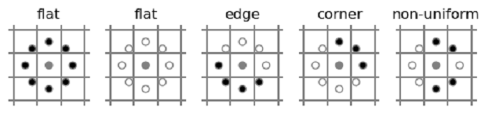
The figure above illustrates results where black (or white) pixels indicate lower (or higher) intensity compared to the central pixel. When all surrounding pixels are uniformly black or white, the image region is flat and lacks distinctive features. Continuous sequences of black or white pixels form "uniform" patterns, which can be interpreted as corners or edges. Patterns that alternate between black and white pixels are categorized as "non-uniform.
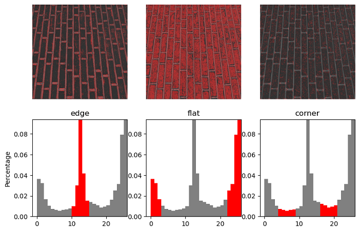
Example
Let's apply the Local Binary Pattern (LBP) to analyze a brick texture. The resulting plot will highlight the flat, edge-like, and corner-like regions within the image.
from skimage.transform import rotate
from skimage.feature import local_binary_pattern
from skimage import data
from skimage.color import label2rgb
import numpy as np
import matplotlib.pyplot as plt

# Define LBP method to 'uniform'
METHOD = 'uniform'

# LBP settings
radius = 3
n_points = 8 * radius

# Function to overlay labels on an image
def overlay_labels(image, lbp, labels):
   mask = np.logical_or.reduce([lbp == each for each in labels])
   return label2rgb(mask, image=image, bg_label=0, alpha=0.5)

# Function to highlight bars in a histogram
def highlight_bars(bars, indexes):
   for i in indexes:
      bars[i].set_facecolor('r')

image = data.brick()
lbp = local_binary_pattern(image, n_points, radius, METHOD)

# Function to plot histograms of LBP of textures
def hist(ax, lbp):
   n_bins = int(lbp.max() + 1)
   return ax.hist(lbp.ravel(), density=True, bins=n_bins, range=(0, n_bins),
      facecolor='0.5')

# Create subplots for image and histograms
fig, (ax_img, ax_hist) = plt.subplots(nrows=2, ncols=3, figsize=(9, 6))
plt.gray()

titles = ('edge', 'flat', 'corner')
w = width = radius - 1
edge_labels = range(n_points // 2 - w, n_points // 2 + w + 1)
flat_labels = list(range(0, w + 1)) + list(range(n_points - w, n_points + 2))
i_14 = n_points // 4            # 1/4th of the histogram
i_34 = 3 * (n_points // 4)      # 3/4th of the histogram
corner_labels = (list(range(i_14 - w, i_14 + w + 1)) +
   list(range(i_34 - w, i_34 + w + 1)))

label_sets = (edge_labels, flat_labels, corner_labels)

# Display labeled images and histograms
for ax, labels in zip(ax_img, label_sets):
   ax.imshow(overlay_labels(image, lbp, labels))

for ax, labels, name in zip(ax_hist, label_sets, titles):
   counts, _, bars = hist(ax, lbp)
   highlight_bars(bars, labels)
   ax.set_ylim(top=np.max(counts[:-1]))
   ax.set_xlim(right=n_points + 2)
   ax.set_title(name)

ax_hist[0].set_ylabel('Percentage')
for ax in ax_img:
   ax.axis('off')
Output