- Computer Graphics - Home
- Computer Graphics Basics
- Computer Graphics Applications
- Graphics APIs and Pipelines
- Computer Graphics Maths
- Sets and Mapping
- Solving Quadratic Equations
- Computer Graphics Trigonometry
- Computer Graphics Vectors
- Linear Interpolation
- Computer Graphics Devices
- Cathode Ray Tube
- Raster Scan Display
- Random Scan Device
- Phosphorescence Color CRT
- Flat Panel Displays
- 3D Viewing Devices
- Images Pixels and Geometry
- Color Models
- Line Generation
- Line Generation Algorithm
- DDA Algorithm
- Bresenham's Line Generation Algorithm
- Mid-point Line Generation Algorithm
- Circle Generation
- Circle Generation Algorithm
- Bresenham's Circle Generation Algorithm
- Mid-point Circle Generation Algorithm
- Ellipse Generation Algorithm
- Polygon Filling
- Polygon Filling Algorithm
- Scan Line Algorithm
- Flood Filling Algorithm
- Boundary Fill Algorithm
- 4 and 8 Connected Polygon
- Inside Outside Test
- 2D Transformation
- 2D Transformation
- Transformation Between Coordinate System
- Affine Transformation
- Raster Methods Transformation
- 2D Viewing
- Viewing Pipeline and Reference Frame
- Window Viewport Coordinate Transformation
- Viewing & Clipping
- Point Clipping Algorithm
- Cohen-Sutherland Line Clipping
- Cyrus-Beck Line Clipping Algorithm
- Polygon Clipping Sutherland–Hodgman Algorithm
- Text Clipping
- Clipping Techniques
- Bitmap Graphics
- 3D Viewing Transformation
- 3D Computer Graphics
- Parallel Projection
- Orthographic Projection
- Oblique Projection
- Perspective Projection
- 3D Transformation
- Rotation with Quaternions
- Modelling and Coordinate Systems
- Back-face Culling
- Lighting in 3D Graphics
- Shadowing in 3D Graphics
- 3D Object Representation
- Represnting Polygons
- Computer Graphics Surfaces
- Visible Surface Detection
- 3D Objects Representation
- Computer Graphics Curves
- Computer Graphics Curves
- Types of Curves
- Bezier Curves and Surfaces
- B-Spline Curves and Surfaces
- Data Structures For Graphics
- Triangle Meshes
- Scene Graphs
- Spatial Data Structure
- Binary Space Partitioning
- Tiling Multidimensional Arrays
- Color Theory
- Colorimetry
- Chromatic Adaptation
- Color Appearance
- Antialiasing
- Ray Tracing
- Ray Tracing Algorithm
- Perspective Ray Tracing
- Computing Viewing Rays
- Ray-Object Intersection
- Shading in Ray Tracing
- Transparency and Refraction
- Constructive Solid Geometry
- Texture Mapping
- Texture Values
- Texture Coordinate Function
- Antialiasing Texture Lookups
- Procedural 3D Textures
- Reflection Models
- Real-World Materials
- Implementing Reflection Models
- Specular Reflection Models
- Smooth-Layered Model
- Rough-Layered Model
- Surface Shading
- Diffuse Shading
- Phong Shading
- Artistic Shading
- Computer Animation
- Computer Animation
- Keyframe Animation
- Morphing Animation
- Motion Path Animation
- Deformation Animation
- Character Animation
- Physics-Based Animation
- Procedural Animation Techniques
- Computer Graphics Fractals
Computer Graphics - 2D Transformation
Transformation means changing some graphics into something else by applying rules. We can have various types of transformations such as translation, scaling up or down, rotation, shearing, etc. When a transformation takes place on a 2D plane, it is called 2D transformation.
Transformations play an important role in computer graphics to reposition the graphics on the screen and change their size or orientation.
Homogenous Coordinates
To perform a sequence of transformation such as translation followed by rotation and scaling, we need to follow a sequential process −
- Translate the coordinates,
- Rotate the translated coordinates, and then
- Scale the rotated coordinates to complete the composite transformation.
To shorten this process, we have to use 3×3 transformation matrix instead of 2×2 transformation matrix. To convert a 2×2 matrix to 3×3 matrix, we have to add an extra dummy coordinate W.
In this way, we can represent the point by 3 numbers instead of 2 numbers, which is called Homogenous Coordinate system. In this system, we can represent all the transformation equations in matrix multiplication. Any Cartesian point P(X, Y) can be converted to homogenous coordinates by P (Xh, Yh, h).
Translation
A translation moves an object to a different position on the screen. You can translate a point in 2D by adding translation coordinate (tx, ty) to the original coordinate (X, Y) to get the new coordinate (X, Y).
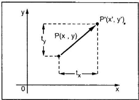
From the above figure, you can write that −
X = X + tx
Y = Y + ty
The pair (tx, ty) is called the translation vector or shift vector. The above equations can also be represented using the column vectors.
$P = \frac{[X]}{[Y]}$ p' = $\frac{[X']}{[Y']}$T = $\frac{[t_{x}]}{[t_{y}]}$
We can write it as −
P = P + T
Rotation
In rotation, we rotate the object at particular angle θ (theta) from its origin. From the following figure, we can see that the point P(X, Y) is located at angle φ from the horizontal X coordinate with distance r from the origin.
Let us suppose you want to rotate it at the angle θ. After rotating it to a new location, you will get a new point P (X, Y).
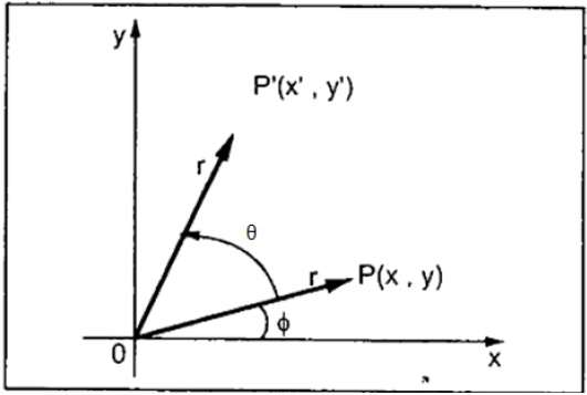
Using standard trigonometric the original coordinate of point P(X, Y) can be represented as −
$X = r \, cos \, \phi ...... (1)$
$Y = r \, sin \, \phi ...... (2)$
Same way we can represent the point P (X, Y) as −
${x}'= r \: cos \: \left ( \phi \: + \: \theta \right ) = r\: cos \: \phi \: cos \: \theta \: − \: r \: sin \: \phi \: sin \: \theta ....... (3)$
${y}'= r \: sin \: \left ( \phi \: + \: \theta \right ) = r\: cos \: \phi \: sin \: \theta \: + \: r \: sin \: \phi \: cos \: \theta ....... (4)$
Substituting equation (1) & (2) in (3) & (4) respectively, we will get
${x}'= x \: cos \: \theta − \: y \: sin \: \theta $
${y}'= x \: sin \: \theta + \: y \: cos \: \theta $
Representing the above equation in matrix form,
$$[X' Y'] = [X Y] \begin{bmatrix} cos\theta & sin\theta \\ −sin\theta & cos\theta \end{bmatrix}OR $$
P = P . R
Where R is the rotation matrix
$$R = \begin{bmatrix} cos\theta & sin\theta \\ −sin\theta & cos\theta \end{bmatrix}$$
The rotation angle can be positive and negative.
For positive rotation angle, we can use the above rotation matrix. However, for negative angle rotation, the matrix will change as shown below −
$$R = \begin{bmatrix} cos(−\theta) & sin(−\theta) \\ -sin(−\theta) & cos(−\theta) \end{bmatrix}$$
$$=\begin{bmatrix} cos\theta & −sin\theta \\ sin\theta & cos\theta \end{bmatrix} \left (\because cos(−\theta ) = cos \theta \; and\; sin(−\theta ) = −sin \theta \right )$$
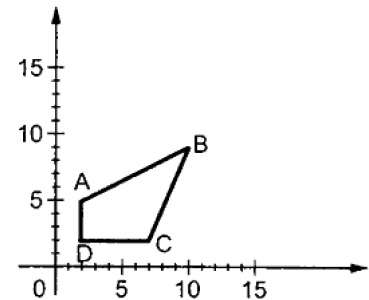
Scaling
To change the size of an object, scaling transformation is used. In the scaling process, you either expand or compress the dimensions of the object. Scaling can be achieved by multiplying the original coordinates of the object with the scaling factor to get the desired result.
Let us assume that the original coordinates are (X, Y), the scaling factors are (SX, SY), and the produced coordinates are (X, Y). This can be mathematically represented as shown below −
X' = X . SX and Y' = Y . SY
The scaling factor SX, SY scales the object in X and Y direction respectively. The above equations can also be represented in matrix form as below −
$$\binom{X'}{Y'} = \binom{X}{Y} \begin{bmatrix} S_{x} & 0\\ 0 & S_{y} \end{bmatrix}$$
OR
P = P . S
Where S is the scaling matrix. The scaling process is shown in the following figure.
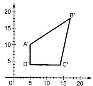
If we provide values less than 1 to the scaling factor S, then we can reduce the size of the object. If we provide values greater than 1, then we can increase the size of the object.
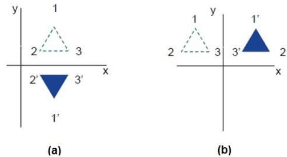
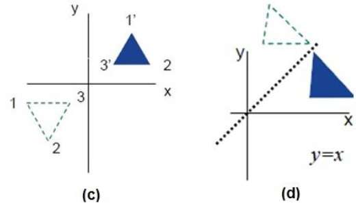
Reflection
Reflection is the mirror image of original object. In other words, we can say that it is a rotation operation with 180°. In reflection transformation, the size of the object does not change.
The following figures show reflections with respect to X and Y axes, and about the origin respectively.
Shear
A transformation that slants the shape of an object is called the shear transformation. There are two shear transformations X-Shear and Y-Shear. One shifts X coordinates values and other shifts Y coordinate values. However; in both the cases only one coordinate changes its coordinates and other preserves its values. Shearing is also termed as Skewing.
X-Shear
The X-Shear preserves the Y coordinate and changes are made to X coordinates, which causes the vertical lines to tilt right or left as shown in below figure.
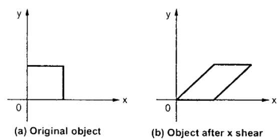
The transformation matrix for X-Shear can be represented as −
$$X_{sh} = \begin{bmatrix} 1& shx& 0\\ 0& 1& 0\\ 0& 0& 1 \end{bmatrix}$$
Y' = Y + Shy . X
X = X
Y-Shear
The Y-Shear preserves the X coordinates and changes the Y coordinates which causes the horizontal lines to transform into lines which slopes up or down as shown in the following figure.
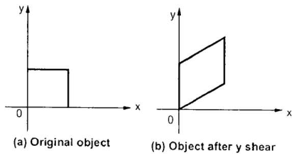
The Y-Shear can be represented in matrix from as −
$$Y_{sh} \begin{bmatrix} 1& 0& 0\\ shy& 1& 0\\ 0& 0& 1 \end{bmatrix}$$
X = X + Shx . Y
Y = Y
Composite Transformation
If a transformation of the plane T1 is followed by a second plane transformation T2, then the result itself may be represented by a single transformation T which is the composition of T1 and T2 taken in that order. This is written as T = T1T2.
Composite transformation can be achieved by concatenation of transformation matrices to obtain a combined transformation matrix.
A combined matrix −
[T][X] = [X] [T1] [T2] [T3] [T4] . [Tn]
Where [Ti] is any combination of
- Translation
- Scaling
- Shearing
- Rotation
- Reflection
The change in the order of transformation would lead to different results, as in general matrix multiplication is not cumulative, that is [A] . [B] [B] . [A] and the order of multiplication. The basic purpose of composing transformations is to gain efficiency by applying a single composed transformation to a point, rather than applying a series of transformation, one after another.
For example, to rotate an object about an arbitrary point (Xp, Yp), we have to carry out three steps −
- Translate point (Xp, Yp) to the origin.
- Rotate it about the origin.
- Finally, translate the center of rotation back where it belonged.